When looking at geographic variation of songs we usually want to compare the spectrograms from different individuals and sites. This can be challenging when working with large numbers of signals, individuals and/or sites. The new warbleR function catalog aims to simplify this task.
This is how it works:
- The function plots a matrix of spectrograms from signals listed in a selection table (a data frame similar to the example data frame
selec.tablein warbleR) - The graphs are saved as image files in the working directory (or path provided)
- Several images are generated if the number of signals don’t fit in a single file
- Spectrograms can be labeled or color tagged to facilitate exploring variation related to the parameter of interest (e.g. site, song type) A legend can be added to help match colors with tag levels and different color palettes can be used for each tag
- The duration of the signals can be “fixed” so all the spectrograms have the same duration (and can be compared more easily)
- Users can control the number of rows and columns as well as the width and height of the output image
Below is a short tutorial showing some of these features. To be able to run the code you need warbleR 1.1.6 or higher, which has not been released on CRAN and it’s only available in the most recent development version on github. It can be installed using the devtools package as follows
#run it only if devtools isn't installed
install.packages("devtools")

devtools::install_github("maRce10/warbleR")
Load the package and save the example sound files as .wav in the working directory
library(warbleR)

data(list = c("Phae.long1", "Phae.long2", "Phae.long3",
              "Phae.long4", "selec.table"))
writeWave(Phae.long1,"Phae.long1.wav")
writeWave(Phae.long2,"Phae.long2.wav")
writeWave(Phae.long3,"Phae.long3.wav")
writeWave(Phae.long4,"Phae.long4.wav")
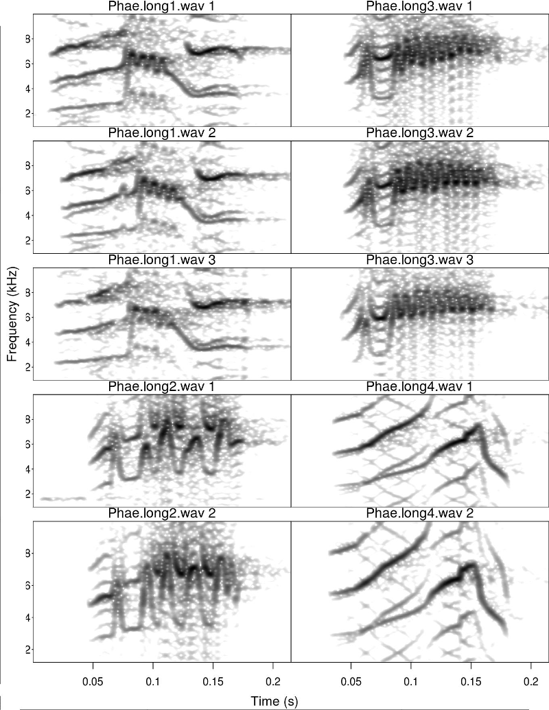
The basic catalog plots the spectrograms of the signals listed in ‘X’. ‘X’ is simply a data frame with the name of sound files and the temporal position of the signals in those sound files (as in the selec.table example data). The following code creates a catalog with 2 columns and 5 rows labeled with the sound file name and selection number (default labels argument)
catalog(X = selec.table[1:10,], flim = c(1, 10), nrow = 5, ncol = 2,
        same.time.scale = TRUE, mar = 0.01, wl = 200, gr = FALSE)
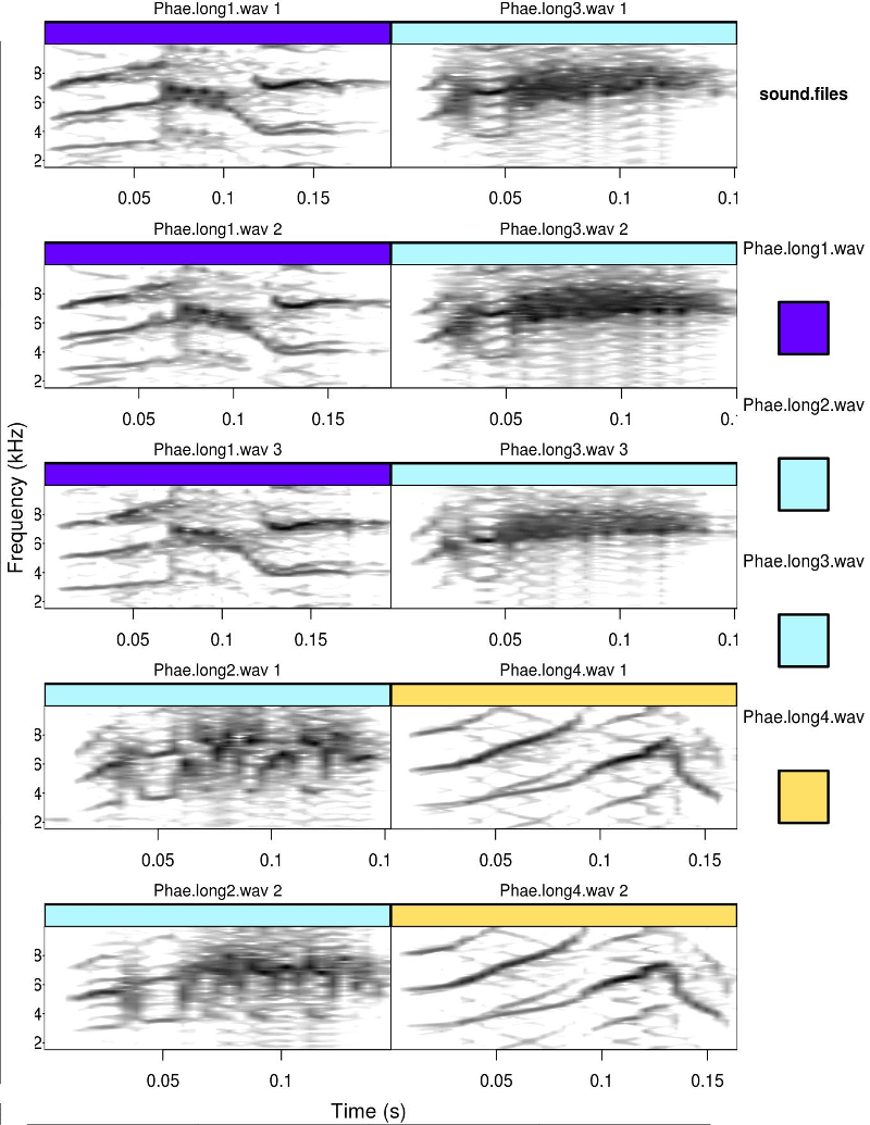
Spectrograms can be color-tagged using the tags argument. A legend is added when legend > 0 (check documentation). The duration can also be allowed to vary between spectrograms setting same.time.scale = TRUE
catalog(X = selec.table[1:10,], flim = c(1, 10), nrow = 5, ncol = 2,
        same.time.scale = FALSE, mar = 0.01, wl = 200, legend = 1,
        tags = c("sound.files"), leg.wd = 10)
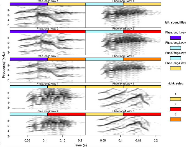
Two color tags can be used at the same times (tags argument) using different color palettes for each tag (tag.pal argument). The code below also uses a different color palette for the spectrogram (pal argument) and set orientation of the output image file to horizontal
catalog(X = selec.table[1:10,], flim = c(1, 10), nrow = 5, ncol = 2,
       mar = 0.01, wl = 200, orientation = "h",  tags = c("sound.files", "selec"),
       leg.wd = 10)
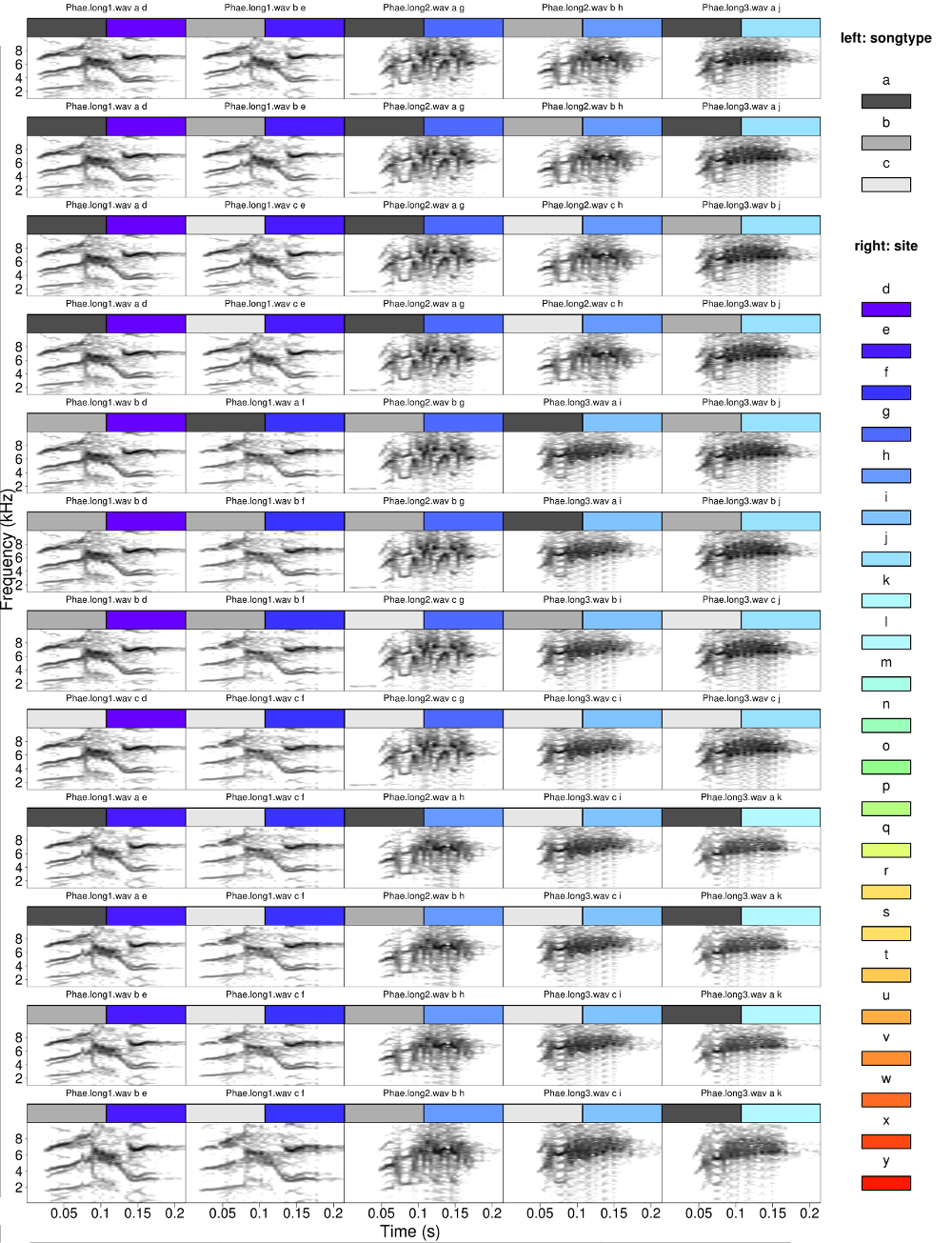
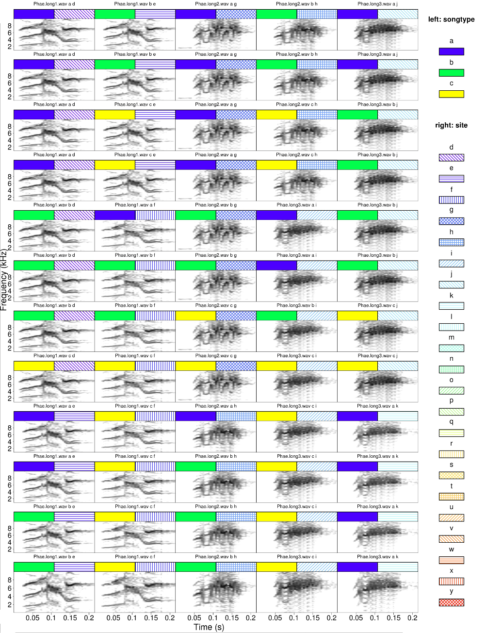
Many more columns and rows can be displayed. In this example a bigger selection data frame is created by combining binding several times the data used in the previous examples. The code also creates some new (hypothetical) data for song type and site> Note that the data is sorted by sites so songs from the same site are closer in the catalog
#create bigger data
Y <- selec.table

for(i in 1:4) Y <- rbind(Y, Y)

#simulated columns
  Y$songtype <- sample(letters[1:3], nrow(Y), replace = T)
  Y$site <- rep(letters[4:25], nrow(Y))[1:nrow(Y)]

  #sort by site and the by song type
Y <- Y[order(Y$site, Y$songtype), ]


catalog(X = Y, flim = c(1, 10), nrow = 12, ncol = 5, cex = 2, leg.wd = 8,
       mar = 0.01, wl = 200, labels = c("sound.files","songtype", "site"),
       legend = 3, width = 23, height = 30,
       tag.pal = list(gray.colors, temp.colors), tags = c("songtype", "site"))
The first image would look like this (several image are produced in the signals don’t fit in a single one)
When several levels are displayed in a tag colors could become very similar, as in the example above. In that case cross-hatched labels can be used using the hatching argument. Either one or both color tags can be cross-hatched. The following applies cross-hatching on the second tag
catalog(X = Y, flim = c(1, 10), nrow = 12, ncol = 5, cex = 2, leg.wd = 8,
        mar = 0.01, wl = 200, legend = 3, width = 23, height = 30,
        tag.pal = list(topo.colors, temp.colors),tags = c("songtype", "site"),
        hatching = 2)
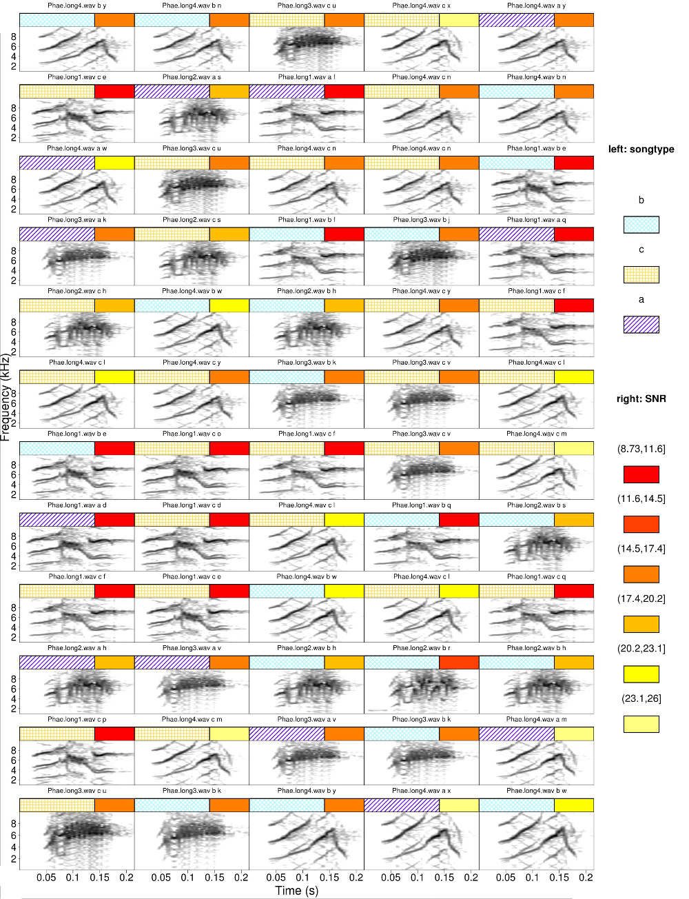
Continuous variables can be used for color tagging as well. The following code calculates the signal-to-noise ratio for each selection and then use it to tag them in the catalog. The breaks argument specifies that the signal-to-noise ratio range should be split in 3 intervals. It also sets the first color tag twice the size of the second one
#get signal-to-noise ratio
Ysnr <- sig2noise(X = Y, mar = 0.04)

#shuffle rows (just for not having snr values unsorted)
set.seed(27)
Ysnr <- Ysnr[sample(1:nrow(Ysnr)),]

catalog(X = Ysnr, flim = c(1, 10), nrow = 12, ncol = 5, cex = 2, leg.wd = 8,
       mar = 0.01, wl = 200, tag.widths = c(2, 1),legend = 3,
 width = 23, height = 30, tag.pal = list(temp.colors, heat.colors),
  tags = c("songtype", "SNR"), hatching = 1, breaks = 3)
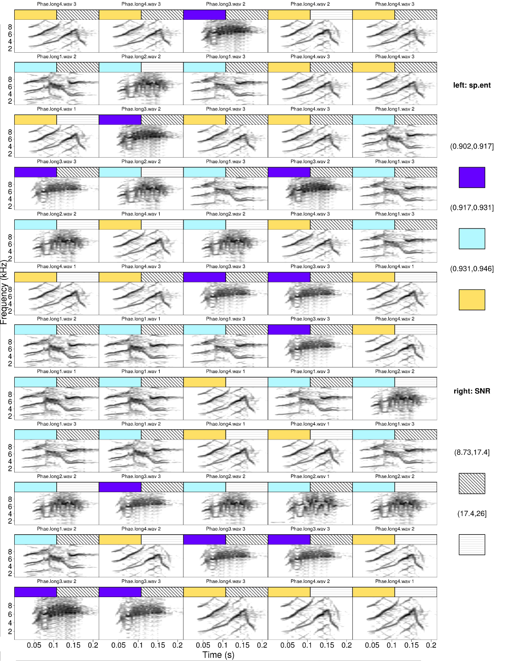
Both tags could be numeric. The following code calculates the spectral entropy with specan and the use it as a tag along with the signal-to-noise ratio
#get signal-to-noise ratio
Ysnr$sp.ent <- specan(X = Ysnr)[,"sp.ent"]

catalog(X = Ysnr, flim = c(1, 10), nrow = 12, ncol = 5, cex = 2, leg.wd = 8,
        mar = 0.01, wl = 200, legend = 3,  width = 23, height = 30, tag.pal = list(temp.colors, gray.colors), tags = c("sp.ent", "SNR"),
        hatching = 2, breaks = c(3, 2))
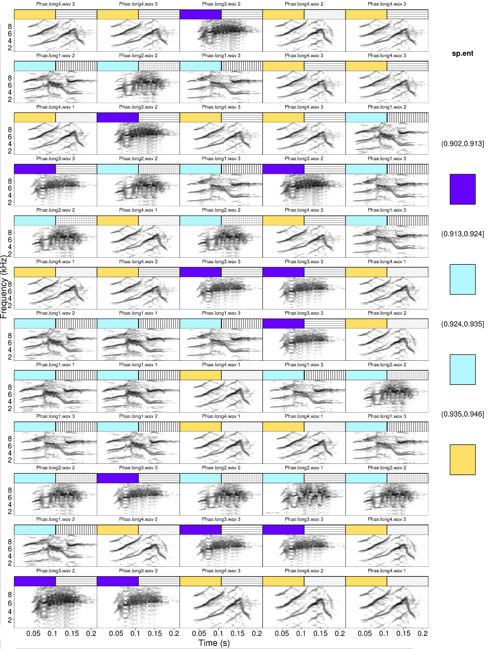
The legend can be removed for one of both tags. The argument legend = 2 plots the legend only for the second tag
catalog(X = Ysnr, flim = c(1, 10), nrow = 12, ncol = 5, cex = 2, leg.wd = 8,
        mar = 0.01, wl = 200, legend = 1,  width = 23, height = 30, tag.pal = list(temp.colors, gray.colors), tags = c("sp.ent", "SNR"), hatching = 2, breaks = 4)
The following plots show a nice example of song geographic variation of Northern Cardinals (Cardinalis cardinalis) in Mexico (from my collaborator Marco Ortiz).


A single pdf containing all catalog images can be generated using the catalog2pdf function.
The catalog function has other arguments to specify spectrogram settings (e.g. margin, grid, frequency limits) and image parameters (e.g. image type, resolution). Check out the function help document.