A [previous post]https://marce10.github.io/coded_bioacoustics/post/2017-03-17-creating_song_catalogs/) described the new function catalog. Here are a few updates on catalog based on suggestions from warbleR users.
To be able to run the code you need warbleR 1.1.9 or higher, which hasn’t been released on CRAN and it’s only available in the most recent development version on github. It can be installed using the devtools package as follows
# install devtools if is not yet installed
if(!"devtools" %in% installed.packages()[,"Package"]) install.packages("devtools")

devtools::install_github("maRce10/warbleR")
And load the package and save the example sound files as .wav in the working directory
library(warbleR)

data(list = c("Phae.long1", "Phae.long2", "Phae.long3",
              "Phae.long4", "selec.table"))
writeWave(Phae.long1,"Phae.long1.wav")
writeWave(Phae.long2,"Phae.long2.wav")
writeWave(Phae.long3,"Phae.long3.wav")
writeWave(Phae.long4,"Phae.long4.wav")
1) Arguments “spec.mar”, “lab.mar”, “max.group.colors” and “group.tag” to color background of selection groups
The following code creates a catalog with 3 columns and 3 rows labeled with the sound file name and selection number (default labels argument)
catalog(X = selec.table[1:9,], flim = c(1, 11), nrow = 3, ncol = 3,
        height = 10, width = 10, same.time.scale = TRUE, mar = 0.01,
        wl = 150, gr = FALSE, box = FALSE)
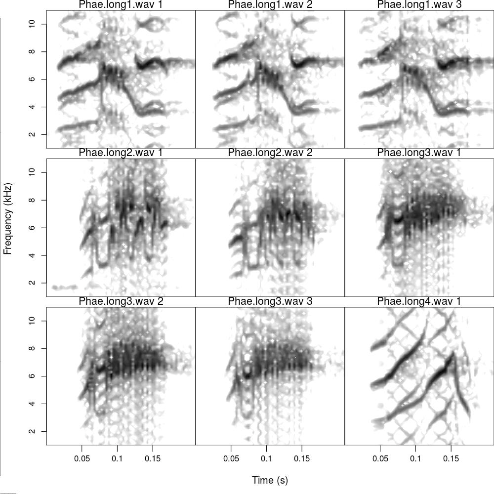
The new arguments can be used to add a background color that is shared by selections belonging to the same grouping variable level. The following code uses the “sound.files” column to color selection groups using “group.tag”. It also makes use of the “spec.mar” to increase the colored areas around the spectrograms and “lab.mar” to shrink the area allocated for selection labels and tags
# modify palette to have softer colors
cmc <- function(n) cm.colors(n, alpha = 0.5)

catalog(X = selec.table[1:9,], flim = c(1, 11), nrow = 3, ncol = 3,
        height = 10, width = 10, tag.pal = list(cmc), cex = 0.8,
        same.time.scale = TRUE, mar = 0.01, wl = 150, gr = FALSE,
        group.tag = "sound.files", spec.mar = 0.4, lab.mar = 0.8, box = FALSE)
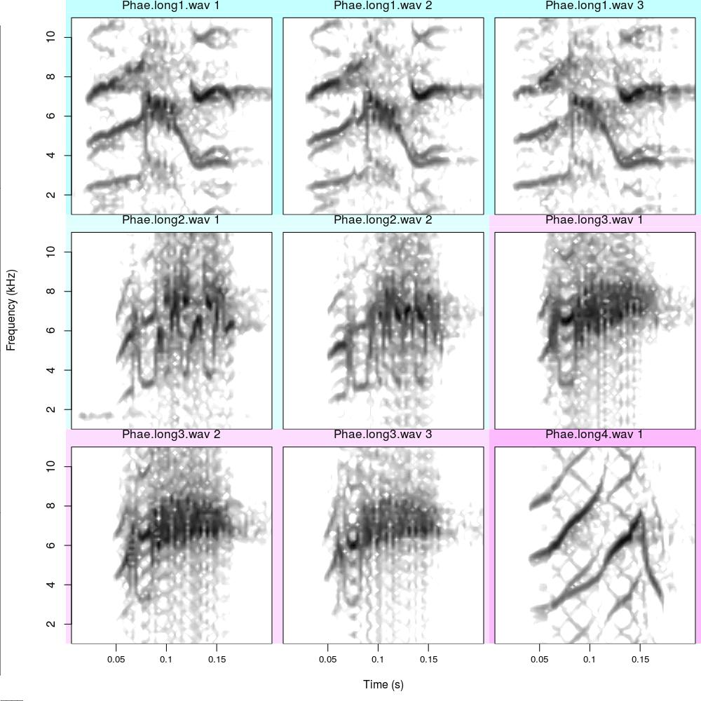
Note that the selection tables are sorted to ensure that selection sharing the same grouping factor level are clumped together in the catalog.
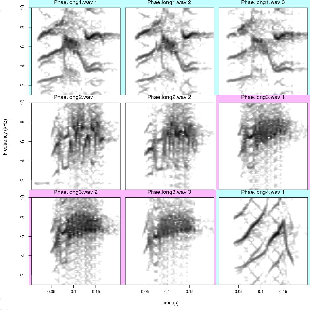
In the example some sound files are highlighted with very similar colors, which makes the visual identification of groups difficult. Using a different palette might solve the problem. Alternatively, the “max.group.cols” argument can be used to set a maximum number of different colors (independent of the levels of the grouping variable) that will be recycled when the number of colors is smaller than the number of levels. This works as follows
catalog(X = selec.table[1:9,], flim = c(1, 10), nrow = 3, ncol = 3,
        height = 10, width = 10, tag.pal = list(cmc), cex = 0.8,
        same.time.scale = TRUE, mar = 0.01, wl = 200, gr = FALSE,
        group.tag = "sound.files", spec.mar = 0.4, lab.mar = 0.8,
        max.group.cols = 3, box = FALSE)
2) Arguments “title”, “by.row”, “prop.mar”, “box” and “rm.axes” to further customize catalog setup
As their names suggest, the arguments “title” and “rm.axes” allow users to add a title at the top of catalogs and remove the x and y axes. respectively:
catalog(X = selec.table[1:9,], flim = c(1, 10), nrow = 3, ncol = 3,
        height = 10, width = 10, tag.pal = list(cmc), cex = 0.8,
        same.time.scale = TRUE, mar = 0.01, wl = 200, gr = FALSE,
        group.tag = "sound.files", spec.mar = 0.4, lab.mar = 0.8,
        max.group.cols = 3, rm.axes = TRUE,
        title = "This one has a title and no axes", box = FALSE)
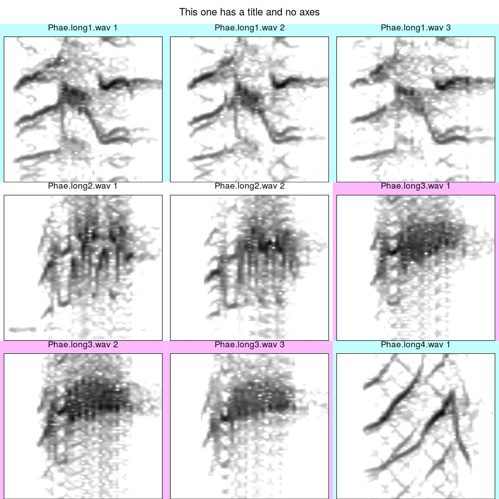
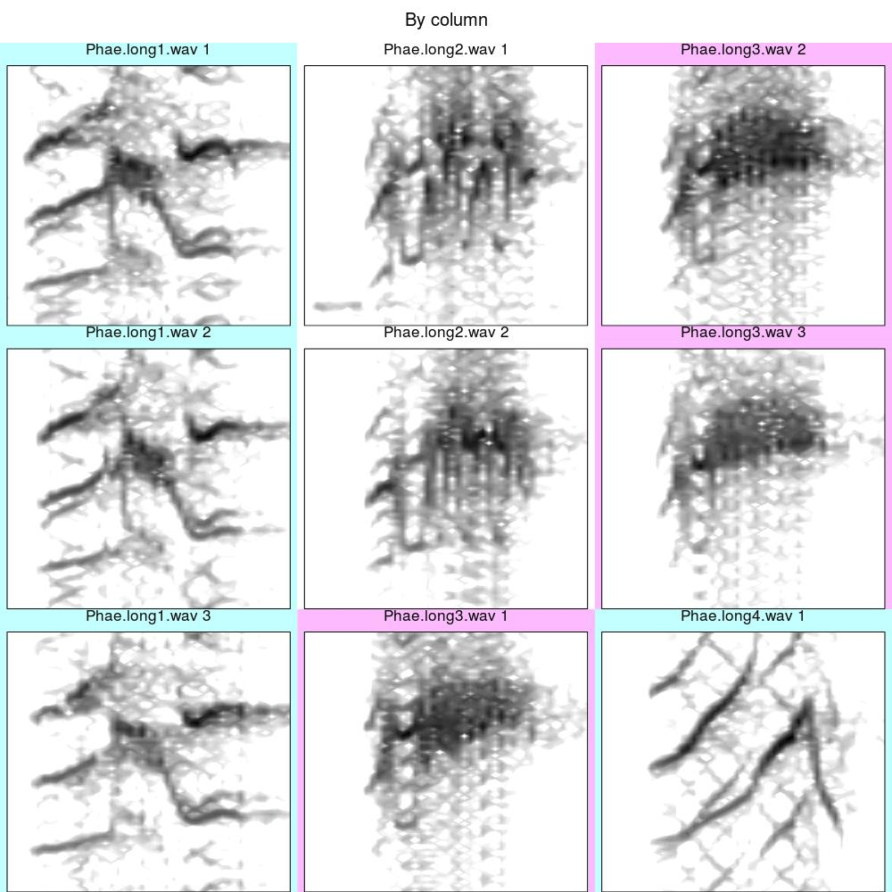
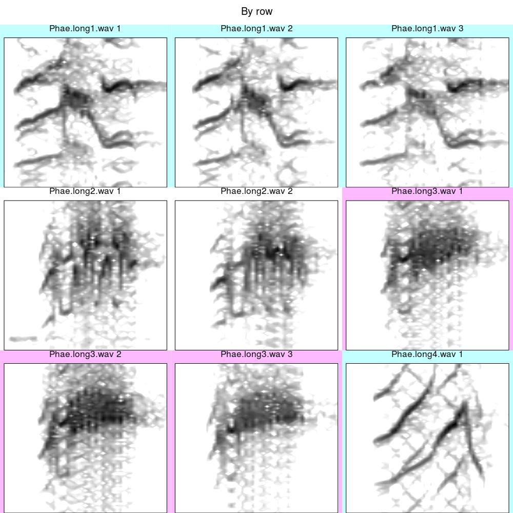
The argument “by.row” allows to fill catalogs either by rows (if TRUE) or by columns (if FALSE).
By column
catalog(X = selec.table[1:9,], flim = c(1, 10), nrow = 3, ncol = 3,
        height = 10, width = 10, tag.pal = list(cmc), cex = 0.8,
        same.time.scale = TRUE, mar = 0.01, wl = 200, gr = FALSE,
        group.tag = "sound.files", spec.mar = 0.4, lab.mar = 0.8,
        max.group.cols = 3, rm.axes = TRUE, title = "By column",
        by.row = FALSE, box = FALSE)
By row
catalog(X = selec.table[1:9,], flim = c(1, 10), nrow = 3, ncol = 3,
        height = 10, width = 10, tag.pal = list(cmc), cex = 0.8,
        same.time.scale = TRUE, mar = 0.01, wl = 200, gr = FALSE,
        group.tag = "sound.files", spec.mar = 0.4, lab.mar = 0.8,
        max.group.cols = 3, rm.axes = TRUE, title = "By row",
        by.row = TRUE, box = FALSE)
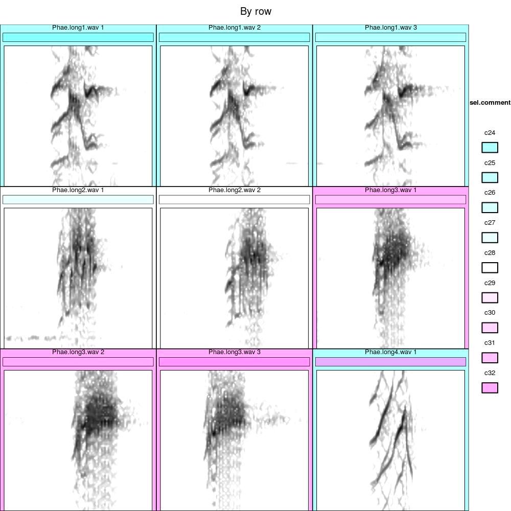
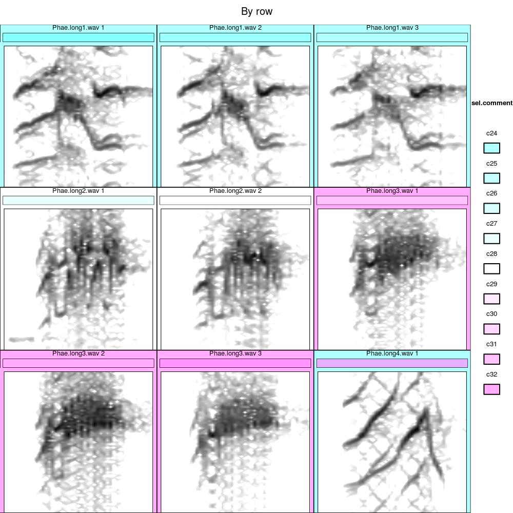
The argument “box” allows users to draw a rectangle around the spectrogram and corresponding labels and tags
catalog(X = selec.table[1:9,], flim = c(1, 10), nrow = 3, ncol = 3,
        height = 10, width = 10, tag.pal = list(cmc), cex = 0.8,
        same.time.scale = TRUE, mar = 0.01, wl = 200, gr = FALSE,
        group.tag = "sound.files", spec.mar = 0.4, lab.mar = 0.8,
        max.group.cols = 3, rm.axes = TRUE, title = "By row",
        by.row = TRUE, tags = "sel.comment", box = TRUE)
Finally, the argument “prop.mar” allows to add margins at both sides of the signals (when creating the spectrogram) that is proportional to the duration of the signal. For instance a value of 0.1 in a signal of 1s will add 0.1 s at the beginning and end of the signal. This can be particularly useful when the duration of signals varies a lot. In this example a margin equals to a third of signal duration is used:
catalog(X = selec.table[1:9,], flim = c(1, 10), nrow = 3, ncol = 3,
        height = 10, width = 10, tag.pal = list(cmc), cex = 0.8,
        same.time.scale = TRUE, mar = 0.01, wl = 200, gr = FALSE,
        group.tag = "sound.files", spec.mar = 0.4, lab.mar = 0.8,
        max.group.cols = 3, rm.axes = TRUE, title = "By row",
        by.row = TRUE, prop.mar = 1/3, tags = "sel.comment", box = TRUE)
