This short post shows how to use the seltailor function to adjust selection frequency and time ‘coordinates’ in an interactive and iterative manner.
To be able to run the code you need warbleR 1.1.9 or higher, which hasn’t been released on CRAN and it’s only available on github. It can be installed using the devtools package as follows
# install devtools and monitor if are not yet installed
# install devtools if is not yet installed
if(!"devtools" %in% installed.packages()[,"Package"]) install.packages("devtools")

devtools::install_github("maRce10/warbleR")
seltailor function
The function aims to provide an easy way to manually fix imperfect selections, as those that in some cases are obtain from automatic detection (e.g. from the autodetec function).
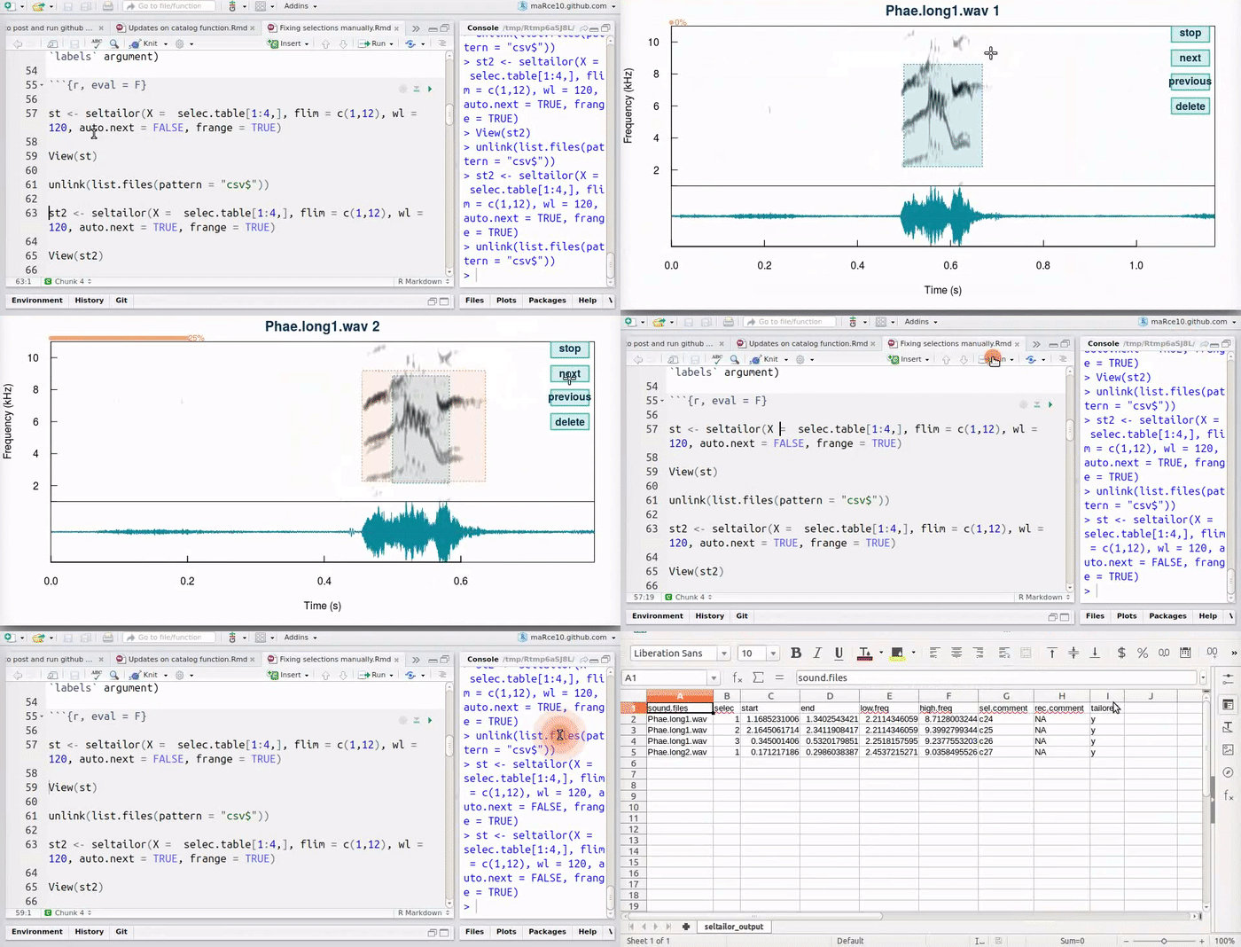
This function produces an interactive spectrographic view in which users can select new time/frequency coordinates the selections. 4 “buttons” are provided at the upper right side of the spectrogram that allow to stop the analysis (“stop”), go to the next sound file (“next”), return to the previous selection (“previous”) or delete the current selection (“delete”). When a unit has been selected, the function plots dotted lines in the start and end of the selection in the spectrogram (or a box if frange = TRUE). Only the last selection is kept for each selection that is adjusted.
The function produces a .csv file (seltailor_output.csv) with the same information than the input data frame, except for the new time coordinates, plus a new column (X$tailored) indicating if the selection has been tailored. The file is saved in the working directory and is updated every time the user moves into the next sound file (next sel “button”) or stop the process (Stop “button”). It also return the same data frame as and object in the R environment. If no selection is made (by clicking on the ’next’ button) the original time/frequency coordinates are kept. When resuming the process (after “stop” and re-running the function in the same working directory), the function will continue working on the selections that have not been analyzed. The function also displays a progress bar right on top of the sepctrogram.
First load the example data and recordings
library(warbleR)

setwd(tempdir())
data(list = c("Phae.long1", "Phae.long2", "Phae.long3",
              "Phae.long4", "selec.table"))
writeWave(Phae.long1,"Phae.long1.wav")
writeWave(Phae.long2,"Phae.long2.wav")
writeWave(Phae.long3,"Phae.long3.wav")
writeWave(Phae.long4,"Phae.long4.wav")
Add some ’noise’ to the selections so they are a bit off the actual song position
selec.table$start <- selec.table$start + rnorm(n = nrow(selec.table), sd = 0.03)
selec.table$end <- selec.table$end + rnorm(n = nrow(selec.table), sd = 0.03)
Now run the function on the selection table. For simplicity, it is run only on the first 4 selections
      flim = c(1,12), wl = 120, auto.next = FALSE,
st <- seltailor(X =  selec.table[1:4,],
      frange = TRUE)

View(st)
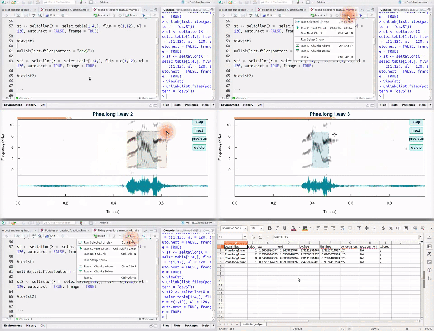
And this is how it works

The auto.next argument can help speed up the process once users feel confortable with the function. The pause argument (not shown) controls how long the function waits until it moves into the next selection
unlink(list.files(pattern = "csv$"))

st2 <- seltailor(X =  selec.table[1:4,],
       flim = c(1,12), wl = 120, auto.next = TRUE,
       frange = TRUE)

View(st2)

The function has many more arguments to customize spectrograms. The index argument can be used to only fix a subset of the signals (while returning the whole data set). Check the function documentation for a full description of the additional arguments.