This post shows how to create and use the new warbleR object class extended_selection_table.
These objects are created with the selec_table() function. The function takes data frames containing selection data (sound file name, selection, start, end …), checks whether the information is consistent (see checksels() function for details) and saves the ‘diagnostic’ metadata as an attribute. When the argument extended = TRUE the function generates an object of class extended_selection_table which also contains a list of wave objects corresponding to each of the selections in the data frame. Hence, the function transforms selection tables into self-contained objects as they no longer need the original sound files for running most acoustic analysis in
warbleR. This can facilitate a lot the storing and sharing of (bio)acoustic data. In addition, it also speeds up processes as sound files do not need to be read every time the data is analyzed.
Let’s first install and/or load warbleR developmental version (if there is an older warbleR version installed it has to be removed first):
# remove warbleR
remove.packages("warbleR")

# install devtools if not installed
if (!"devtools" %in% installed.packages()[,"Package"])
  install.packages("devtools")

# and install warbleR from github
devtools::install_github("maRce10/warbleR")

# load warbleR
library(warbleR)
… set a temporary folder, load the example sound files and set warbleR options (see warbleR_options() documentation):
# set temporary directory
setwd(tempdir())

# load example data
data(list = c("Phae.long1", "Phae.long2", "Phae.long3", "Phae.long4",
              "selec.table"))

# save recordings as wave files
writeWave(Phae.long1,"Phae.long1.wav")
writeWave(Phae.long2,"Phae.long2.wav")
writeWave(Phae.long3,"Phae.long3.wav")
writeWave(Phae.long4,"Phae.long4.wav")

# set warbleR options
warbleR_options(wl = 300, pb = FALSE,
          parallel = parallel::detectCores() - 1)
Now, as mentioned above, you need the selec_table() function to create extended selection table. You also need to set the the argument extended = TRUE (otherwise the class would be a “selection_table”). Here the example data that comes with warbleR is used as the data frame to be converted to an object of class extended_selection_table:
selec.table
The following code converts it to an extended selection table:
# make extended selection table
ext_st <- selection_table(X = selec.table, pb = FALSE,
          extended = TRUE, confirm.extended = FALSE)
And that’s it. Now the acoustic data and the selection data (as well as the additional metadata) are all together in a single R object.
Manipulating extended selection tables
Several functions can be used to deal with objects of this class. You can test if the object belongs to the extended_selection_table:
is_extended_selection_table(ext_st)
[1] TRUE
You can subset the selection in the same way that any other data frame in it will maintain its attributes:
ext_st2 <- ext_st[1:2, ]

is_extended_selection_table(ext_st2)
[1] TRUE
There is also a generic version of print() for these class of objects:
## print
print(ext_st)
object of class 'extended_selection_table'
 contains a selection table data frame with 11 rows and 9 columns:
       sound.files channel selec start     end bottom.freq top.freq sel.comment rec.comment
1 Phae.long1.wav_1       1     1   0.1 0.27303      2.2201   8.6044         c24          NA
2 Phae.long1.wav_2       1     1   0.1 0.26305      2.1694   8.8071         c25          NA
3 Phae.long1.wav_3       1     1   0.1 0.27492      2.2183   8.7566         c26          NA
4 Phae.long2.wav_1       1     1   0.1 0.23257      2.3169   8.8223         c27          NA
5 Phae.long2.wav_2       1     1   0.1 0.22615      2.2840   8.8880         c28          NA
6 Phae.long3.wav_1       1     1   0.1 0.23122      3.0068   8.8223         c29          NA
... and 5 more rows
11 wave objects (as attributes):
[1] "Phae.long1.wav_1" "Phae.long1.wav_2" "Phae.long1.wav_3" "Phae.long2.wav_1" "Phae.long2.wav_2"
[6] "Phae.long3.wav_1"
... and 5 more
and a data frame (check.results) generated by checkres() (as attribute)
the selection table was created by element (see 'class_extended_selection_table')
## which is the same than this
ext_st
object of class 'extended_selection_table'
 contains a selection table data frame with 11 rows and 9 columns:
       sound.files channel selec start     end bottom.freq top.freq sel.comment rec.comment
1 Phae.long1.wav_1       1     1   0.1 0.27303      2.2201   8.6044         c24          NA
2 Phae.long1.wav_2       1     1   0.1 0.26305      2.1694   8.8071         c25          NA
3 Phae.long1.wav_3       1     1   0.1 0.27492      2.2183   8.7566         c26          NA
4 Phae.long2.wav_1       1     1   0.1 0.23257      2.3169   8.8223         c27          NA
5 Phae.long2.wav_2       1     1   0.1 0.22615      2.2840   8.8880         c28          NA
6 Phae.long3.wav_1       1     1   0.1 0.23122      3.0068   8.8223         c29          NA
... and 5 more rows
11 wave objects (as attributes):
[1] "Phae.long1.wav_1" "Phae.long1.wav_2" "Phae.long1.wav_3" "Phae.long2.wav_1" "Phae.long2.wav_2"
[6] "Phae.long3.wav_1"
... and 5 more
and a data frame (check.results) generated by checkres() (as attribute)
the selection table was created by element (see 'class_extended_selection_table')
You can also row-bind them together. Here the original extended_selection_table is split into 2 and bind back together using rbind():
ext_st3 <- ext_st[1:5, ]

ext_st4 <- ext_st[6:11, ]

ext_st5 <- rbind(ext_st3, ext_st4)

#print
ext_st5
object of class 'extended_selection_table'
 contains a selection table data frame with 11 rows and 9 columns:
       sound.files channel selec start     end bottom.freq top.freq sel.comment rec.comment
1 Phae.long1.wav_1       1     1   0.1 0.27303      2.2201   8.6044         c24          NA
2 Phae.long1.wav_2       1     1   0.1 0.26305      2.1694   8.8071         c25          NA
3 Phae.long1.wav_3       1     1   0.1 0.27492      2.2183   8.7566         c26          NA
4 Phae.long2.wav_1       1     1   0.1 0.23257      2.3169   8.8223         c27          NA
5 Phae.long2.wav_2       1     1   0.1 0.22615      2.2840   8.8880         c28          NA
6 Phae.long3.wav_1       1     1   0.1 0.23122      3.0068   8.8223         c29          NA
... and 5 more rows
11 wave objects (as attributes):
[1] "Phae.long1.wav_1" "Phae.long1.wav_2" "Phae.long1.wav_3" "Phae.long2.wav_1" "Phae.long2.wav_2"
[6] "Phae.long3.wav_1"
... and 5 more
and a data frame (check.results) generated by checkres() (as attribute)
the selection table was created by element (see 'class_extended_selection_table')
# the same than the original one
all.equal(ext_st, ext_st5)
[1] TRUE
The wave objects can be indvidually read using read_sound_file(), a wrapper on tuneR’s readWave() function, that can take extended selection tables:
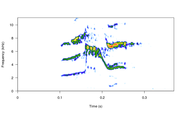
wv1 <- read_sound_file(X = ext_st, index = 3, from = 0, to = 0.37)
These are regular wave objects:
class(wv1)
[1] "Wave"
attr(,"package")
[1] "tuneR"
wv1
Wave Object
	Number of Samples:      8325
	Duration (seconds):     0.37
	Samplingrate (Hertz):   22500
	Channels (Mono/Stereo): Mono
	PCM (integer format):   TRUE
	Bit (8/16/24/32/64):    16
spectro(wv1, wl = 150, grid = FALSE, scale = FALSE, ovlp = 90)
par(mfrow = c(3, 2), mar = rep(0, 4))

for(i in 1:6){

  wv <- read_sound_file(X = ext_st, index = i, from = 0.05, to = 0.32)

  spectro(wv, wl = 150, grid = FALSE, scale = FALSE, axisX = FALSE,
          axisY = FALSE, ovlp = 90)

}
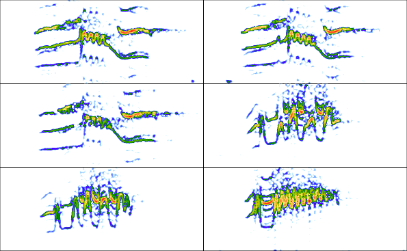
The read_sound_file() function takes the table as well as the index of the selection to be read (e.g. the row number).
Keep in mind that is likely that other functions that modify data frames will remove the attributes in which wave objects and metadata are stored. For instances, merging and extended selection table will get rid of its attributes:
# create a new data frame
Y <- data.frame(sound.files = ext_st$sound.files, site = "La Selva", lek = c(rep("SUR", 5), rep("CCL", 6)))

# merge
mrg_ext_st <- merge(ext_st, Y, by = "sound.files")

# check class
is_extended_selection_table(mrg_ext_st)
[1] FALSE
In this case we can use the fix_extended_selection_table() function to transfer the attributes from the original extended selection table:
# fix
mrg_ext_st <- fix_extended_selection_table(X = mrg_ext_st, Y = ext_st)

# check class
is_extended_selection_table(mrg_ext_st)
[1] TRUE
This works as long as some of the original sound files are kept and no other selections are added.
Object size
Extended selection table size will be a function of the number of selections, sampling rate, selection duration and margin duration (the margin is how much extra time you want to keep at each side of the selection). In this example a data frame with 1000 selections is created just by repeating the example data frame several times and then converted to an extended selection table:
lng.selec.table <- do.call(rbind, replicate(100, selec.table,
                        simplify = FALSE))[1:1000,]

lng.selec.table$selec <- 1:nrow(lng.selec.table)

nrow(lng.selec.table)

lng_ext_st <- selection_table(X = lng.selec.table, pb = FALSE,
                        extended = TRUE, confirm.extended = FALSE)

lng_ext_st
object of class 'extended_selection_table'
 contains a selection table data frame with 1000 rows and 9 columns:
       sound.files channel selec start     end bottom.freq top.freq sel.comment rec.comment
1 Phae.long1.wav_1       1     1   0.1 0.27303      2.2201   8.6044         c24          NA
2 Phae.long1.wav_2       1     1   0.1 0.26305      2.1694   8.8071         c25          NA
3 Phae.long1.wav_3       1     1   0.1 0.27492      2.2183   8.7566         c26          NA
4 Phae.long2.wav_4       1     1   0.1 0.23257      2.3169   8.8223         c27          NA
5 Phae.long2.wav_5       1     1   0.1 0.22615      2.2840   8.8880         c28          NA
6 Phae.long3.wav_6       1     1   0.1 0.23122      3.0068   8.8223         c29          NA
... and 994 more rows
1000 wave objects (as attributes):
[1] "Phae.long1.wav_1" "Phae.long1.wav_2" "Phae.long1.wav_3" "Phae.long2.wav_4" "Phae.long2.wav_5"
[6] "Phae.long3.wav_6"
... and 994 more
and a data frame (check.results) generated by checkres() (as attribute)
the selection table was created by element (see 'class_extended_selection_table')
format(object.size(lng_ext_st), units = "auto")
[1] "31.3 Mb"
As you can see the object size is only ~31 MB. So, as a guide, a selection table with 1000 selections similar to those in ‘selec.table’ (mean duration ~0.15 seconds) at 22.5 kHz sampling rate and the default margin (mar = 0.1) will generate an extended selection table of ~31 MB or ~310 MB for a 10000 row selection table.
Running analysis on extended selection tables
These objects can be used as input for most warbleR functions. We need to delete the sound files in order to show the data is actually contained in the new objects:
list.files(pattern = "\\.wav$")
[1] "Phae.long1.wav" "Phae.long2.wav" "Phae.long3.wav" "Phae.long4.wav"
# delete files (be careful not to run this
# if you have sound files in the working directory!)
unlink(list.files(pattern = "\\.wav$"))

list.files(pattern = "\\.wav$")
character(0)
Here are a few examples of warbleR functions using extended_selection_table:
Spectral parameters
# spectral parameters
sp <- specan(ext_st)

sp
Cross correlation
xc <- xcorr(ext_st, bp = c(1, 11))

xc
Signal-to-noise ratio
# signal-to-noise ratio
snr <- sig2noise(ext_st, mar = 0.05)

snr
Dynamic time warping distance
dtw.dist <- dfDTW(ext_st, img = FALSE)

dtw.dist
calculating DTW distances (step 2 of 2, no progress bar):
Performance
Using extended_selection_table objects can improve performance (in our case measured as time). Here we used the microbenchmark to compare the performance of sig2noise() and ggplot2 to plot the results. We also need to save the wave files again to be able to run the analysis with regular data frames:
# save recordings as wave files
writeWave(Phae.long1,"Phae.long1.wav")
writeWave(Phae.long2,"Phae.long2.wav")
writeWave(Phae.long3,"Phae.long3.wav")
writeWave(Phae.long4,"Phae.long4.wav")

#run this one if microbenchmark is not installed
# install.packages("microbenchmark")
library(microbenchmark)

# install.packages("ggplot2")
library(ggplot2)

# use only 1 core
warbleR_options(parallel = 1, pb = FALSE)

# use the first 100 selection for the long selection tables
mbmrk.snr <- microbenchmark(extended = sig2noise(lng_ext_st[1:100, ],
      mar = 0.05), regular = sig2noise(lng.selec.table[1:100, ],
                    mar = 0.05), times = 50)

autoplot(mbmrk.snr) + ggtitle("sig2noise")
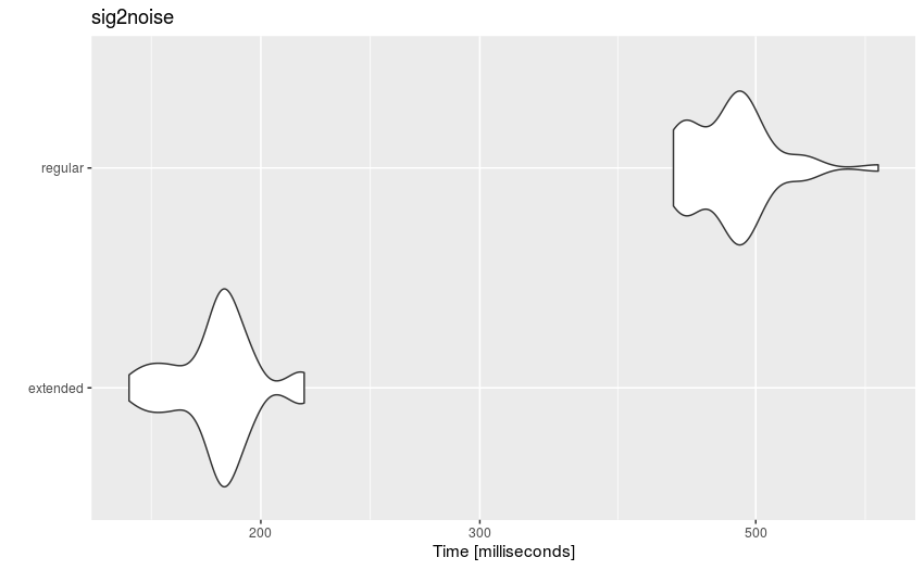
Distribution of sig2noise() timing on regular and extended selection tables
The function runs much faster on extended selection tables. The gain in performance is likely to improve when using longer recordings and data sets (i.e. compensate for computing overhead).
By song
The extended selection tables above were all made ‘by selection’. This is, each sound file inside the object contains a single selection (i.e. 1:1 correspondence between selections and wave objects). Extended selection tables, however, can also be created by using a higher hierarchical level with the argument by.song. In this case, ‘song’ represents a higher level that contains one or more selections and that the user may want to keep together for some particular analysis (e.g. gap duration). The argument by.song takes the name of the character or factor column with the IDs of the different “songs” within a sound file (note that the function assumes that a given song can only be found in a single sound file so selections with the same song ID but from different sound files is taken as different ‘songs’).
For the sake of the example, let’s add an artificial song column to our example data set in which each sound files 2 songs:
# add column
selec.table$song <- c(1, 1, 2, 1, 2, 1, 1, 2, 1, 2, 2)
The data frame looks like this:
Now we can create an extended selection table ‘by song’ using the name of the ‘song’ column (which in this silly example is also ‘song’) as the input for the by.song argument:
bs_ext_st <- selection_table(X = selec.table, extended = TRUE,
                              confirm.extended = FALSE, by.song = "song")
In this case we should only have 8 wave objects instead of 11 as when the object was created ‘by selection’:
# by element
length(attr(ext_st, "wave.objects"))
[1] 11
# by song
length(attr(bs_ext_st, "wave.objects"))
[1] 8
Again, these objects can also be used on further analysis:
# signal-to-noise ratio
bs_snr <- sig2noise(bs_ext_st, mar = 0.05)
The margin would be an important parameter to take into consideration for some downstream functions like those producing plots or using additional time segments around selection to run analysis (e.g. sig2noise() or xcorr()).
Sharing acoustic data
The new object class allows to share complete data sets, including the acoustic data. For instance, with the following code you can download a subset of the data used in Araya-Salas et al (2017) (it can also be downloaded here):
URL <- "https://marceloarayasalas.weebly.com/uploads/2/5/5/2/25524573/extended.selection.table.araya-salas.et.al.2017.bioacoustics.100.sels.rds"

dat <- readRDS(gzcon(url(URL)))

nrow(dat)
[1] 100
format(object.size(dat), units = "auto")
[1] "10.1 Mb"
The total size of the 100 sound files from which these selections were taken adds up to 1.1 GB. The size of the extended selection table is just 10.1 MB.
This data is ready to be used:
sp <- specan(dat, bp = c(2, 10))

head(sp)
And the spectrograms can be displayed:
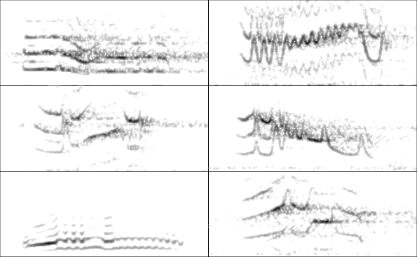
par(mfrow = c(3, 2), mar = rep(0, 4))

for(i in 1:6){

  wv <- read_sound_file(X = dat, index = i, from = 0.17, to = 0.4)

  spectro(wv, wl = 250, grid = FALSE, scale = FALSE, axisX = FALSE,
          axisY = FALSE, ovlp = 90, flim = c(0, 12),
          palette = reverse.gray.colors.1)
}
The ability to compress large data sets and the easiness of conducting analyses requiring only a single R object can potentially simplify data sharing and the reproducibility of bioacoustic analyses.
Please report any bugs here.
Session information
R version 3.4.4 (2018-03-15)
Platform: x86_64-pc-linux-gnu (64-bit)
Running under: Ubuntu 16.04.5 LTS

Matrix products: default
BLAS: /usr/lib/openblas-base/libblas.so.3
LAPACK: /usr/lib/libopenblasp-r0.2.18.so

locale:
 [1] LC_CTYPE=en_US.UTF-8       LC_NUMERIC=C               LC_TIME=en_US.UTF-8        LC_COLLATE=en_US.UTF-8
 [5] LC_MONETARY=en_US.UTF-8    LC_MESSAGES=en_US.UTF-8    LC_PAPER=en_US.UTF-8       LC_NAME=C
 [9] LC_ADDRESS=C               LC_TELEPHONE=C             LC_MEASUREMENT=en_US.UTF-8 LC_IDENTIFICATION=C

attached base packages:
[1] stats     graphics  grDevices utils     datasets  methods   base

other attached packages:
[1] ggplot2_3.0.0        microbenchmark_1.4-4 kableExtra_0.9.0     knitr_1.20           warbleR_1.1.15
[6] NatureSounds_1.0.0   seewave_2.1.0        tuneR_1.3.3          maps_3.3.0

loaded via a namespace (and not attached):
 [1] rgl_0.95.1441        Rcpp_0.12.18         fftw_1.0-4           assertthat_0.2.0     rprojroot_1.3-2
 [6] digest_0.6.16        R6_2.2.2             plyr_1.8.4           Sim.DiffProc_4.1     backports_1.1.2
[11] signal_0.7-6         evaluate_0.11        pracma_2.1.5         httr_1.3.1           highr_0.7
[16] pillar_1.3.0         rlang_0.2.2          lazyeval_0.2.1       curl_3.2             rstudioapi_0.7
[21] rmarkdown_1.10       devtools_1.13.6      moments_0.14         readr_1.1.1          stringr_1.3.1
[26] RCurl_1.95-4.11      munsell_0.5.0        proxy_0.4-22         compiler_3.4.4       Deriv_3.8.5
[31] pkgconfig_2.0.2      htmltools_0.3.6      tidyselect_0.2.4     tibble_1.4.2         dtw_1.20-1
[36] bioacoustics_0.1.5   viridisLite_0.3.0    crayon_1.3.4         dplyr_0.7.6          withr_2.1.2
[41] MASS_7.3-50          bitops_1.0-6         grid_3.4.4           gtable_0.2.0         git2r_0.23.0
[46] magrittr_1.5         scales_1.0.0         stringi_1.2.4        pbapply_1.3-4        scatterplot3d_0.3-41
[51] bindrcpp_0.2.2       xml2_1.2.0           rjson_0.2.20         iterators_1.0.10     tools_3.4.4
[56] glue_1.3.0           purrr_0.2.5          hms_0.4.2            jpeg_0.1-8           parallel_3.4.4
[61] yaml_2.2.0           colorspace_1.3-2     soundgen_1.3.1       rvest_0.3.2          memoise_1.1.0
[66] bindr_0.1.1