We are often interested in getting the frequency range of acoustic signals, either because we have specific predictions about its variation or simply because we want to measure other stuff within that range. Measuring frequency range is typically done by drawing boxes in Raven/Avisoft/Syrinx. An alternative way, and potentially less subjective, is to infer the range from the energy distribution in the frequency domain applying amplitude thresholds on spectrums. I have added two new functions to warbleR that do exactly that:
freq_range_detec: detects the frequency range of signals in wave objects (like a seewave function). Can produce images n the graphic device ifplot = TRUE.freq_range: appliesfreq_range_deteciteratively on signals listed in a selection table (like most warbleR functions). Ifimg = TRUEimage files including a spectrogram and a frequency spectrum are produced for each selection.
This post shows how these functions work.
Let’s first Load/install warbleR:
if(!require(githubinstall)) install.packages("githubinstall")

githubinstall("warbleR", ask = FALSE)

library("warbleR")
We will run the functions on signals detected on a recording from a male Striped-throated Hermit (Phaethornis striigularis) from Xeno-Canto. We can download the sound file and convert it into wave format as follows:
# set temporary working directory
 setwd(tempdir())

# Query and download  Xeno-Canto for metadata using genus and species as keywords
Phae.stri <- quer_xc(qword = "nr:154074", download = TRUE, pb = FALSE)

# Convert mp3 to wav format
# Simultaneously lower sampling rate to speed up down stream analyses
mp32wav(samp.rate = 22.05, pb = FALSE)
Now, we need to detect the time “coordinates” of the signals in the sound file using auto_detec:
ad <- auto_detec(wl = 200, threshold = 3.5, ssmooth = 1200, bp = c(4, 9.6),
                 pb = FALSE,  mindur = 0.1, maxdur = 0.25, img = FALSE)
And selec the highest signal-to-noise ratio signals (just for the sake of the example):
snr <- sig2noise(ad, pb = FALSE, mar = 0.05)

ad <- snr[rank(-snr$SNR) < 60, ]
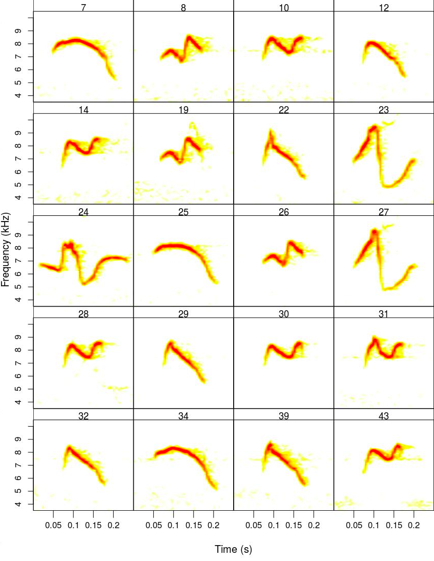
Let’s take a look at the subset of signals that we will analyze (the output of catalog will be found in your working directory):
catalog(ad, nrow = 5, ncol = 4, mar = 0.01, flim = c(3.5, 10.5),
        labels = "selec", pal = reverse.heat.colors, pb = FALSE)

open_wd()

freq_range_detec
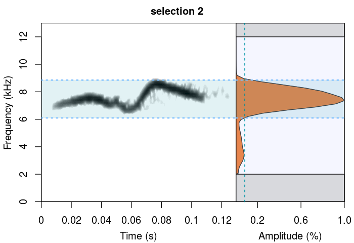
Now we are ready to run the new functions. freq_range_detec works on wave objects. In this example we use it to detect the frequency range of the first selection in “ad”. But first the selection has to be read as a wave object into R:
w2 <- readWave(as.character(ad$sound.files[2]), from = ad$start[2],
               to = ad$end[2], units = "seconds")

freq_range_detec(w2, bp = c(2, 9.6), fsmooth = 1, ovlp = 95,
                 wl = 200, threshold = 8)

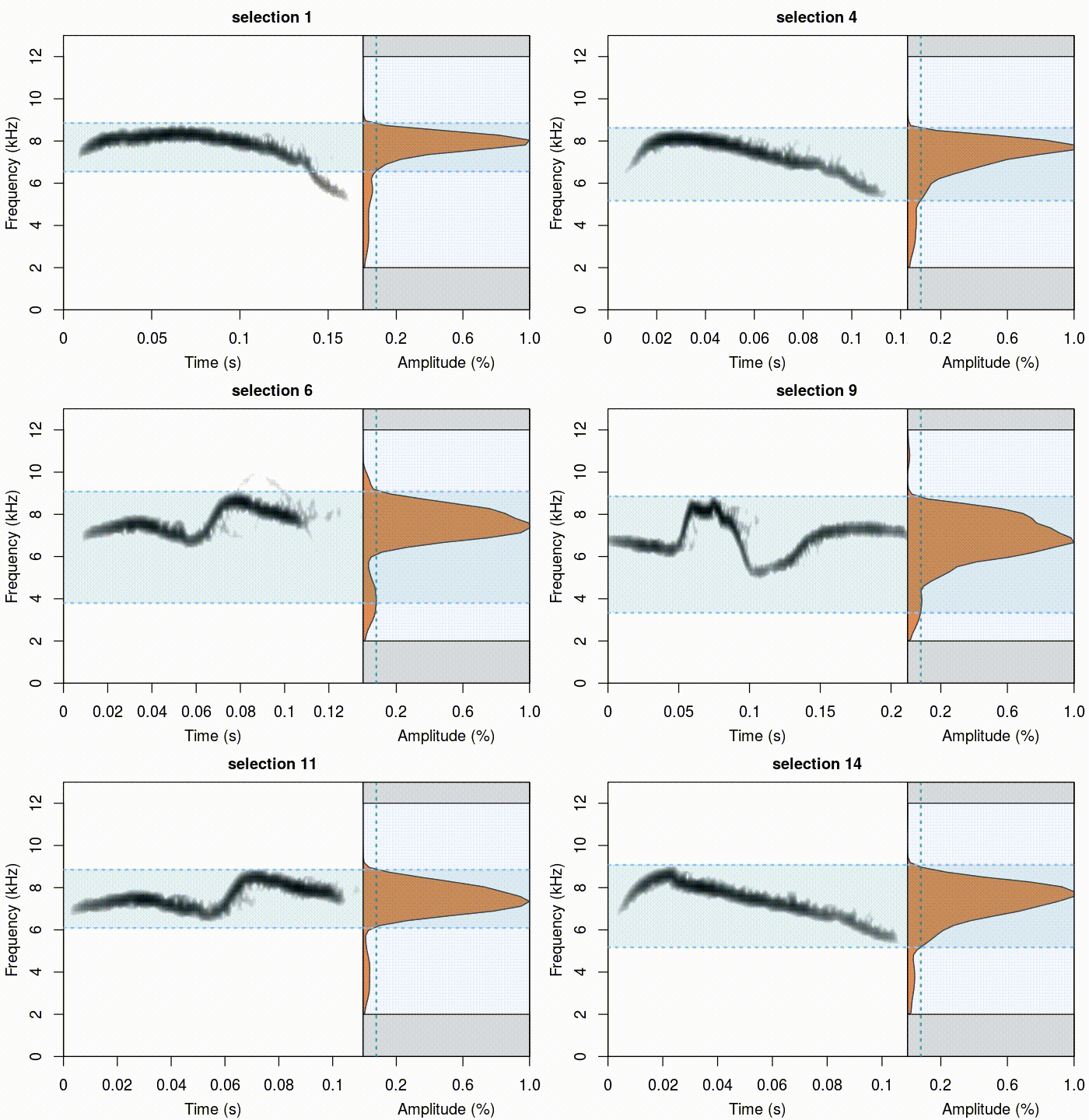
We can look at the detection for each selection in the ‘ad’ data frame using a loop as follows:
for(i in 1:nrow(ad))
{
  wv <- readWave(as.character(ad$sound.files[i]), from = ad$start[i],
                 to = ad$end[i], units = "seconds")

freq_range_detec(wv, bp = c(2, 12), fsmooth = 1, ovlp = 95, wl = 200,
                 threshold = 8, flim = c(0, 13),
                 main = paste("selection", i))

Sys.sleep(0.8)
}

In most cases the detection is good. However, there are some issues with highly amplitude-modulated signals (e.g. high variation in amplitude across the signal). Some parameter tweeking will be required to improve those detections.
freq_range
As mentioned above, the frequency range can be calculated for all selection in a selection table using freq_range:
fr_ad <- freq_range(X = ad, bp = c(2, 12), fsmooth = 0.001, ovlp = 95,
                          wl = 200, threshold = 10, img = FALSE)

View(fr_ad)
The range can then be used as a band pass filter in other warbleR functions like trackfreqs, dfts or specan:
sp <- specan(X = fr_ad, wl = 200, bp = "frange", ovlp = 90, pb = FALSE,
             threshold = 15)

View(sp)
That’s it!