I got the following question about dynamic time warping on frequency contours:
“what I am looking for is to use ffDTW on a file in which I have a column for the filename and then 20 pitch measurements for each of 10000 files (e.g. 10000 rows). Do you have suggestions?”
There is a workaround in warbleR to do that:
The function dfDTW() has the argument ts.df (for time series data frame) that allows to input your own frequency contours (or any other sequences of values taken along the signals).
Let’s first set up the example data and global options:
# load warbleR
library(warbleR)

#load data and save sound files
data(list = c("Phae.long1", "Phae.long2","lbh_selec_table"))
writeWave(Phae.long2, "Phae.long2.wav") #save sound files
writeWave(Phae.long1, "Phae.long1.wav")

# set warbleR global options, including the number of frequency values for contours
# this options can also be set within the function call
warbleR_options(flim = c(1, 12), bp = c(2, 9), wl = 300, pb = FALSE,
                length.out = 30, ovlp = 90)
This is how it works. We will use dfts() to extract dominant frequency contours on the warbleR example data and then input those contours into dfDTW() using the ts.df argument:
# get dom freq contours (will use only the first 5 rows)
cntours <- dfts(X = lbh_selec_table[1:5, ])

# calculate DTW pairwise distances
dfDTW(ts.df = cntours)
##                  Phae.long1.wav-1 Phae.long1.wav-2 Phae.long1.wav-3
## Phae.long1.wav-1            0.000            8.796           15.450
## Phae.long1.wav-2            8.796            0.000           11.719
## Phae.long1.wav-3           15.450           11.719            0.000
## Phae.long2.wav-1           18.779           24.377           22.085
## Phae.long2.wav-2           23.523           35.624           21.585
##                  Phae.long2.wav-1 Phae.long2.wav-2
## Phae.long1.wav-1           18.779           23.523
## Phae.long1.wav-2           24.377           35.624
## Phae.long1.wav-3           22.085           21.585
## Phae.long2.wav-1            0.000           13.868
## Phae.long2.wav-2           13.868            0.000
That output matrix contains the pairwise DTW distance based on our own frequency contours. The data frame containing the contours must have columns for ‘sound.files’ and ‘selec’.
We could even calculate DTW distances based on spectral entropy contours using the sp.en.ts() function:
# get dom freq contours (will use only the first 5 rows)
sp.en.cntours <- sp.en.ts(X = lbh_selec_table[1:5, ])

# calculate DTW pairwise distances
dfDTW(ts.df = sp.en.cntours)
##                  Phae.long1.wav-1 Phae.long1.wav-2 Phae.long1.wav-3
## Phae.long1.wav-1            0.000            0.808            1.007
## Phae.long1.wav-2            0.808            0.000            1.137
## Phae.long1.wav-3            1.007            1.137            0.000
## Phae.long2.wav-1            2.943            2.299            1.997
## Phae.long2.wav-2            1.412            1.359            1.229
##                  Phae.long2.wav-1 Phae.long2.wav-2
## Phae.long1.wav-1            2.943            1.412
## Phae.long1.wav-2            2.299            1.359
## Phae.long1.wav-3            1.997            1.229
## Phae.long2.wav-1            0.000            1.859
## Phae.long2.wav-2            1.859            0.000
Note that, we are using dfDTW() instead of ffDTW() as in the original question. This is because the ts.df argument is only found in dfDTW(). These two functions will be merged at some point in the future anyways.
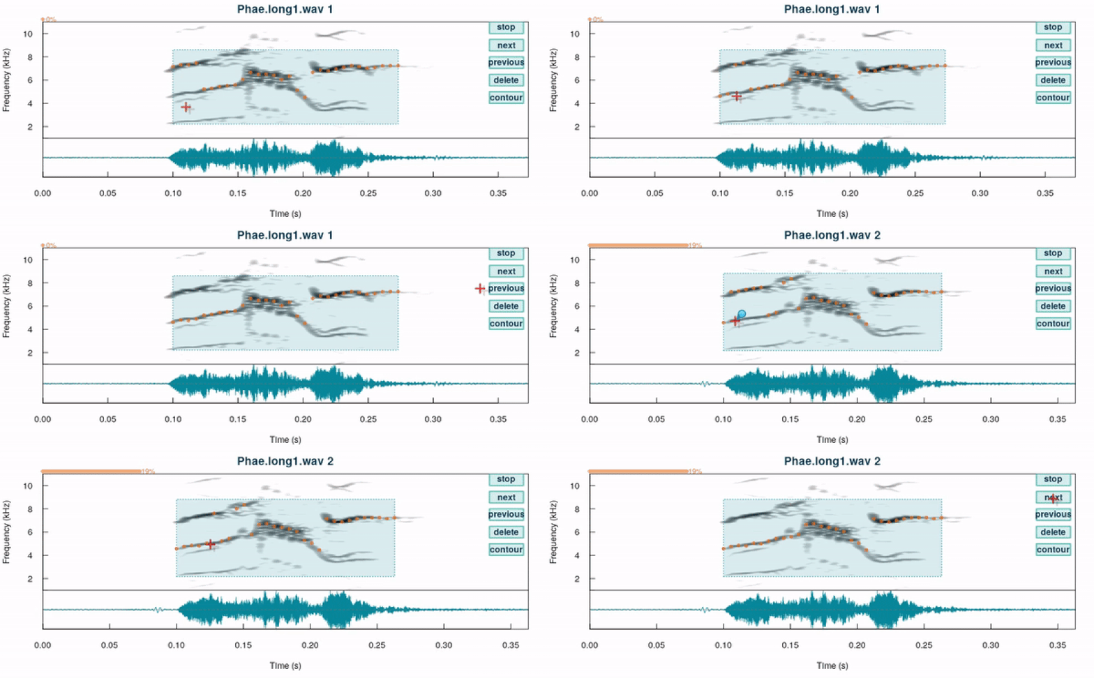
This trick could be particularly useful when the contours have been measured somewhere else or when they need to be manually tailored. The tailoring of frequency contours can be done using seltailor() and the ts.df argument as follows:
tail.cntours <-seltailor(X = lbh_selec_table[1:5, ], ts.df = cntours,
                auto.contour = TRUE)

These signals are far from ideal to do frequency contour tracking, but they help to make the point. As you can see, this is an interactive function in which the user can adjust the frequency of specific points by clicking on the desired frequency. More details about the function can be found on this post and in the function’s documentation.
Hope that helps!
Session information
## R version 3.5.1 (2018-07-02)
## Platform: x86_64-pc-linux-gnu (64-bit)
## Running under: Ubuntu 18.10
##
## Matrix products: default
## BLAS: /usr/lib/x86_64-linux-gnu/openblas/libblas.so.3
## LAPACK: /usr/lib/x86_64-linux-gnu/libopenblasp-r0.3.3.so
##
## locale:
##  [1] LC_CTYPE=en_US.UTF-8       LC_NUMERIC=C
##  [3] LC_TIME=en_US.UTF-8        LC_COLLATE=en_US.UTF-8
##  [5] LC_MONETARY=en_US.UTF-8    LC_MESSAGES=en_US.UTF-8
##  [7] LC_PAPER=en_US.UTF-8       LC_NAME=C
##  [9] LC_ADDRESS=C               LC_TELEPHONE=C
## [11] LC_MEASUREMENT=en_US.UTF-8 LC_IDENTIFICATION=C
##
## attached base packages:
## [1] stats     graphics  grDevices utils     datasets  methods   base
##
## other attached packages:
## [1] warbleR_1.1.16     NatureSounds_1.0.1 seewave_2.1.0
## [4] tuneR_1.3.3        maps_3.3.0
##
## loaded via a namespace (and not attached):
##  [1] knitr_1.20       magrittr_1.5     Sim.DiffProc_4.3 MASS_7.3-50
##  [5] Deriv_3.8.5      rjson_0.2.20     jpeg_0.1-8       pbapply_1.3-4
##  [9] stringr_1.3.1    highr_0.7        tools_3.5.1      parallel_3.5.1
## [13] dtw_1.20-1       iterators_1.0.10 yaml_2.2.0       soundgen_1.3.2
## [17] bitops_1.0-6     RCurl_1.95-4.11  signal_0.7-6     evaluate_0.11
## [21] proxy_0.4-22     stringi_1.2.4    pracma_2.2.2     compiler_3.5.1
## [25] fftw_1.0-4