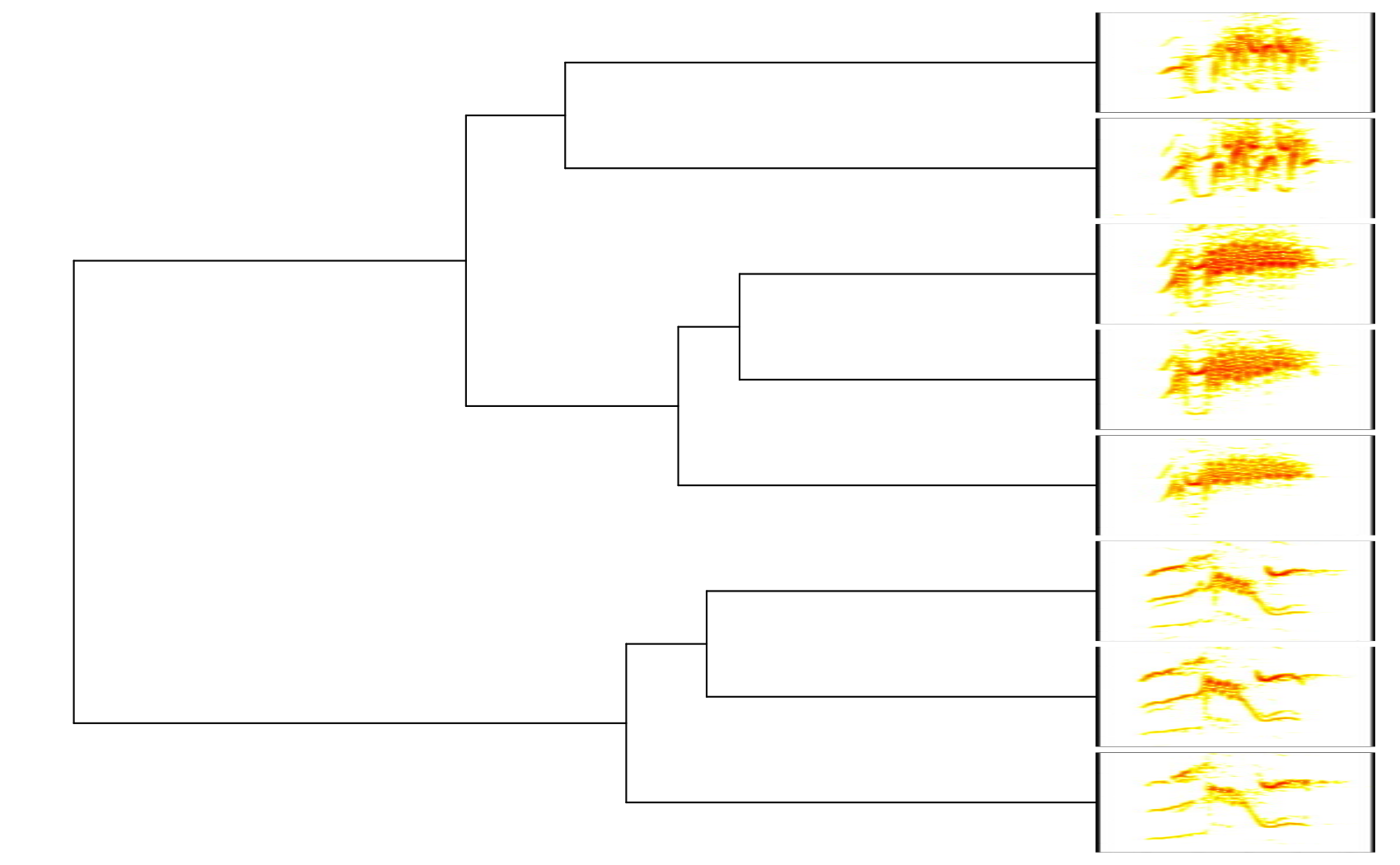
This post describes the new warbleR function phylo_spectro. The function adds spectrograms of sounds annotated in a selection table (‘X argument) onto the tips of a tree (of class ‘phylo’). The ’tip.label’ column in ‘X’ is used to match spectrograms and tree tips. The function uses internally the plot.phylo function from the ape package to plot the tree and warbleR’s specreator function to create the spectrograms. Arguments for both of these functions can be provided for further customization.
We’ll first load the example data set from warbleR as well as the ape package.
# load warbleR and ape
library(warbleR)
library(ape)

#load data and save sound files
data(list = c("Phae.long1", "Phae.long2", "Phae.long3", "lbh_selec_table"))
writeWave(Phae.long1,"Phae.long1.wav")
writeWave(Phae.long2,"Phae.long2.wav")
writeWave(Phae.long3,"Phae.long3.wav")

# set warbleR global options
# this options can also be set within the function call
warbleR_options(wl = 300, pb = FALSE, ovlp = 95, flim = "frange",
                pal = reverse.heat.colors, parallel = 3)
The tricky part is that the selection table must contain a column named ’tip.label’ that matches the tip labels in the tree. The following code calculates pairwise cross-correlations and creates a tree that clusters songs based on cross-correlation dissimilarities (1 - XC scores).
# extract the first 8 rows in the example data
X <- lbh_selec_table[1:8, ]

# add tip.label column
X$tip.label <- paste0(X$sound.files, "-", X$selec)

# run cross correlation
xc <- xcorr(X)

# create a hierarchical cluster
xc.tree <- hclust(d = as.dist(1 - xc))

# convert h clust to phylogenetic tree
xc.tree <- as.phylo(xc.tree)

# plot tree with spectrograms
phylo_spectro(X = X, tree = xc.tree, offset = 0, par.mar = c(1, 1, 1, 8),
inner.mar = rep(0, 4), size = 1, xl = 0.1, show.tip.label = FALSE,
res = 300)
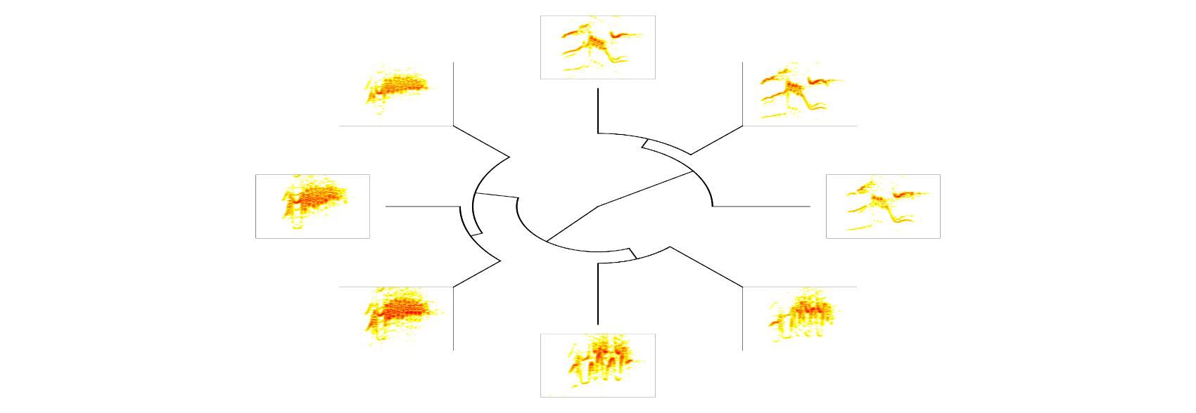
It can also plot fan trees by setting type = "fan":
# plot fan tree with spectrograms
phylo_spectro(X = X, tree = xc.tree, offset = 0.12, par.mar = rep(5, 4),
inner.mar = rep(0, 4), size = 2, type = "fan", show.tip.label = FALSE,
res = 300)
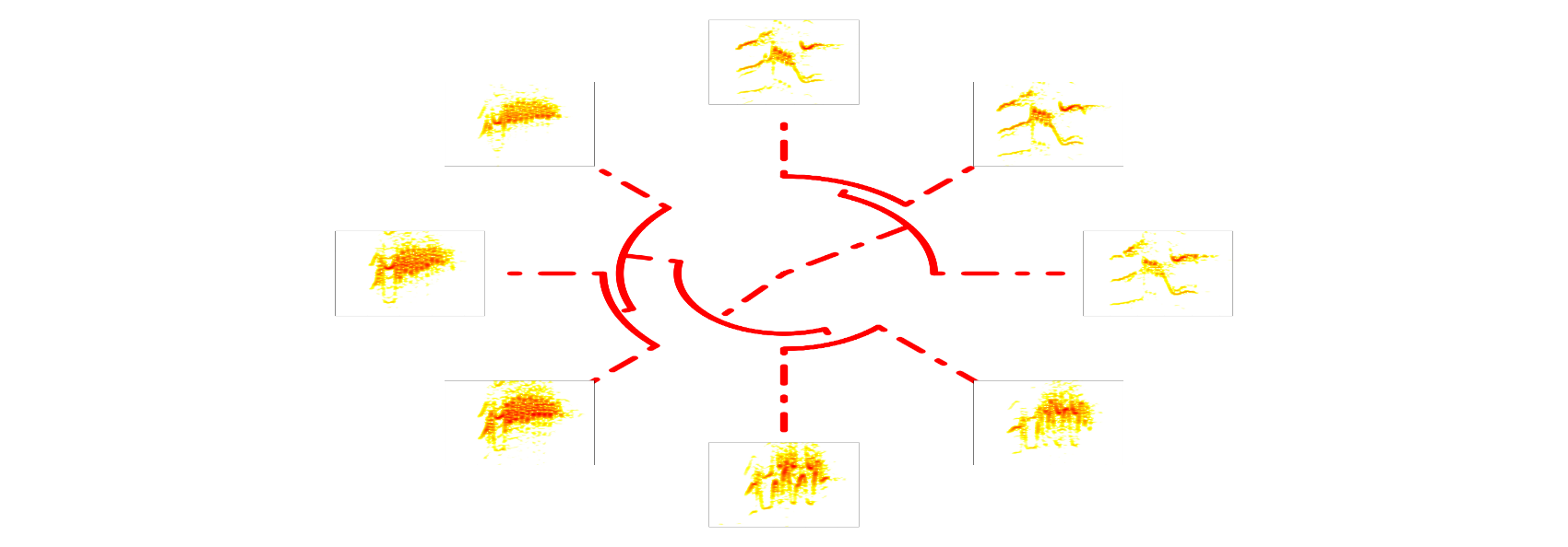
Additional arguments can be passed to plot.phylo. Here we modify ’edge.lty’ and ’edge.witdth’:
# plot tree with spectrograms
phylo_spectro(X = X, tree = xc.tree, offset = 0.12, par.mar = rep(5, 4),
inner.mar = rep(0, 4), size = 2, type = "fan", show.tip.label = FALSE,
res = 300, edge.color = "red", edge.lty = 4, edge.width = 4)
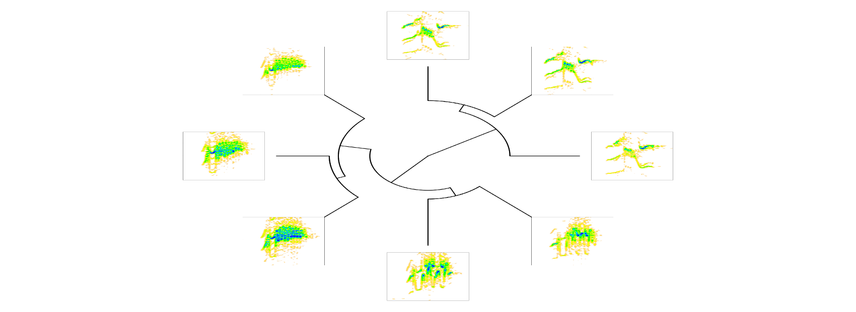
and to specreator. Here we modify ‘pal’ (color palette):
# plot tree with spectrograms
phylo_spectro(X = X, tree = xc.tree, offset = 0.12, par.mar = rep(5, 4),
inner.mar = rep(0, 4), size = 2, type = "fan", show.tip.label = FALSE,
pal = reverse.topo.colors, res = 300)
Here is another example using an extended selection table and more signals:
data("Phae.long.est")

# get songs belonging to 4 different song types
X <- Phae.long.est[c(1:5, 11:15, 21:25, 31:35), ]

# add tip.label column
X$tip.label <- paste0(X$sound.files, "-", X$selec)

# run cross correlation
xc <- xcorr(X)

# create a hierarchical cluster
xc.tree <- hclust(d = as.dist(1 - xc))

# convert h clust to phylogenetic tree
xc.tree <- as.phylo(xc.tree)

# plot fan tree with spectrograms
phylo_spectro(X = X, tree = xc.tree, offset = 0.02, par.mar = rep(2, 4),
inner.mar = rep(0, 4), size = 2.3, type = "fan", res = 300,
show.tip.label = FALSE, pal = reverse.gray.colors.1,
flim = c(2, 10), edge.color = "orange",  edge.width = 3)
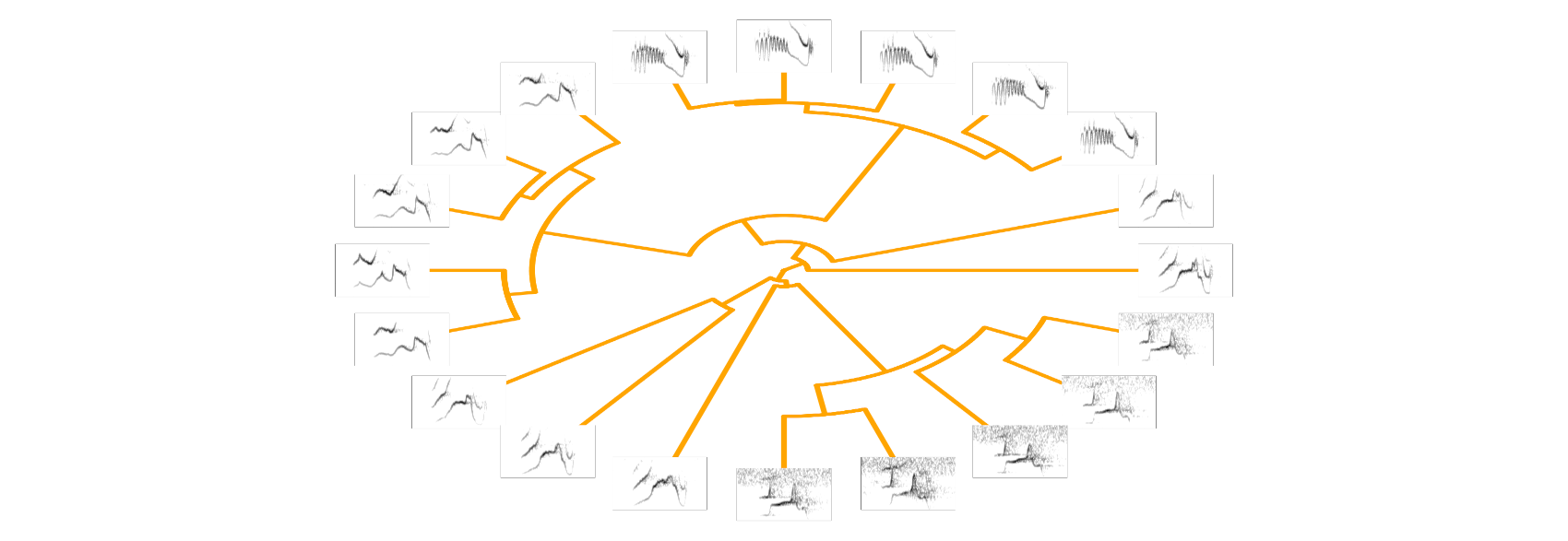
Of course, the function can also plot species songs on phylogenetic trees. Here is an example from an ongoing project:
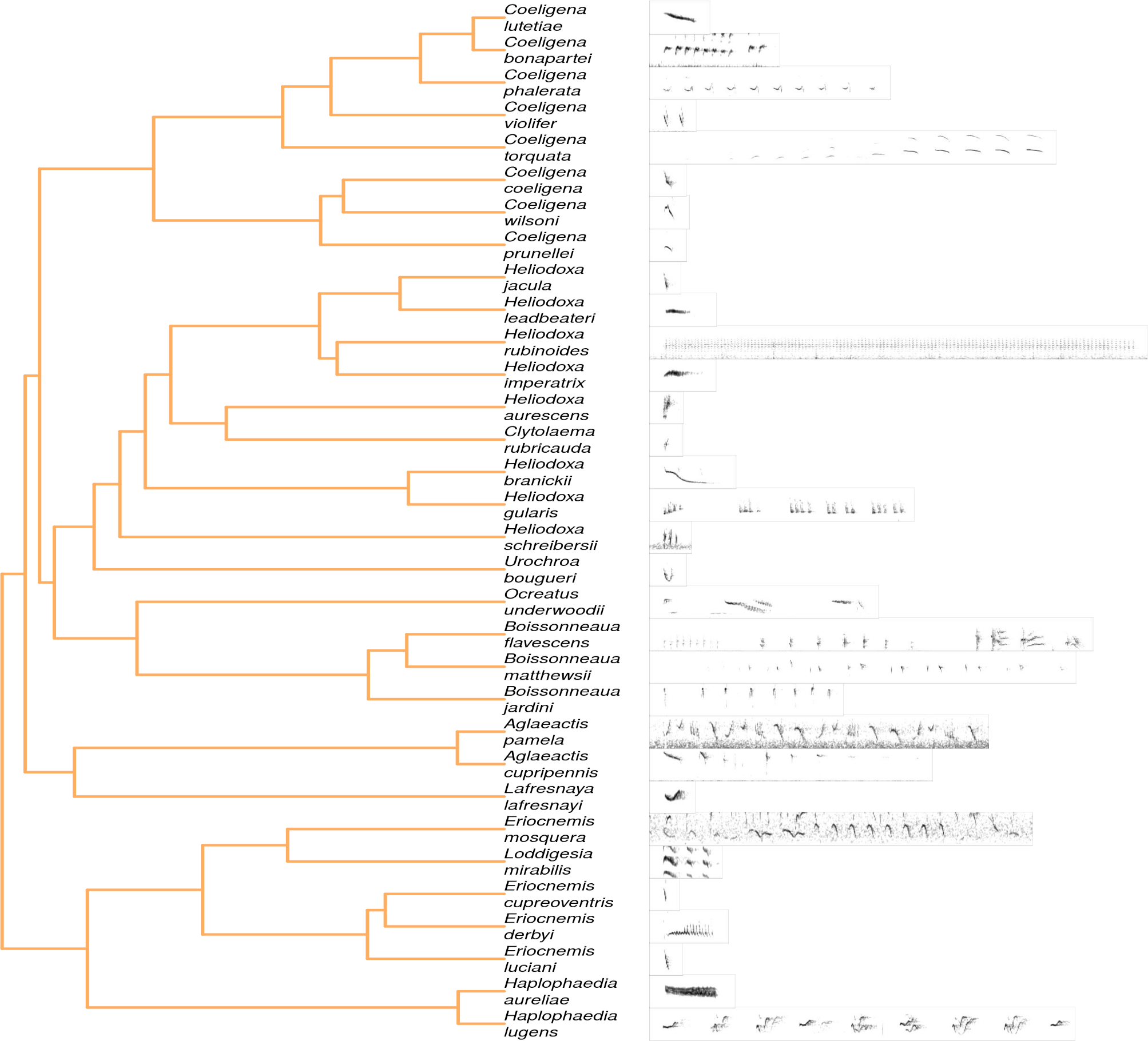
That’s it! Special thanks to Gerardo Soto and Russel Ligon for suggestions on how to make this function work.
Session information
## R version 3.5.1 (2018-07-02)
## Platform: x86_64-pc-linux-gnu (64-bit)
## Running under: Ubuntu 18.10
##
## Matrix products: default
## BLAS: /usr/lib/x86_64-linux-gnu/openblas/libblas.so.3
## LAPACK: /usr/lib/x86_64-linux-gnu/libopenblasp-r0.3.3.so
##
## locale:
##  [1] LC_CTYPE=en_US.UTF-8       LC_NUMERIC=C
##  [3] LC_TIME=en_US.UTF-8        LC_COLLATE=en_US.UTF-8
##  [5] LC_MONETARY=en_US.UTF-8    LC_MESSAGES=en_US.UTF-8
##  [7] LC_PAPER=en_US.UTF-8       LC_NAME=C
##  [9] LC_ADDRESS=C               LC_TELEPHONE=C
## [11] LC_MEASUREMENT=en_US.UTF-8 LC_IDENTIFICATION=C
##
## attached base packages:
## [1] stats     graphics  grDevices utils     datasets  methods   base
##
## other attached packages:
## [1] ape_5.2            warbleR_1.1.16     NatureSounds_1.0.1
## [4] seewave_2.1.0      tuneR_1.3.3        maps_3.3.0
##
## loaded via a namespace (and not attached):
##  [1] Rcpp_1.0.0       knitr_1.20       magrittr_1.5     Sim.DiffProc_4.3
##  [5] MASS_7.3-50      lattice_0.20-35  Deriv_3.8.5      rjson_0.2.20
##  [9] jpeg_0.1-8       pbapply_1.3-4    highr_0.7        stringr_1.3.1
## [13] tools_3.5.1      grid_3.5.1       parallel_3.5.1   nlme_3.1-137
## [17] dtw_1.20-1       iterators_1.0.10 yaml_2.2.0       soundgen_1.3.2
## [21] bitops_1.0-6     RCurl_1.95-4.11  signal_0.7-6     evaluate_0.12
## [25] proxy_0.4-22     stringi_1.2.4    pracma_2.2.2     compiler_3.5.1
## [29] fftw_1.0-4