“Is there a simple way to remove noise from the clips in an extended table – I can do this by directly manipulating the attributes of the table but it seems a bit kludgy … so again, am I missing something simple?”
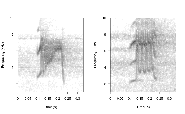
Manipulating clips from extended selection tables can be pretty straightforward. It can be done by using lapply() to go over each clip. Things should be fine as long as you don’t mess with any time related feature (i.e. the time position of the signals in the clip remains unchanged). For example filtering out low frequencies on the clips from the example extended selection table ’lbh.est’ from the package NatureSounds. This is how the original clips look like:
# load packages
library(NatureSounds)
library(warbleR)
library(seewave)

# load data
data("lbh.est")

# extract 2 clips
w1 <- read_wave(lbh.est, 12, from = 0, to = Inf)
w2 <- read_wave(lbh.est, 20, from = 0, to = Inf)

# split graphic device
par(mfrow = c(1, 2))

# plot spectros
spectro(w1, wl = 300, ovlp = 95, flim = c(1, 10), scale = FALSE,
        grid = FALSE, palette = reverse.gray.colors.1,
        collevels = seq(-70, 0, 5))

spectro(w2, wl = 300, ovlp = 95, flim = c(1, 10), scale = FALSE,
        grid = FALSE, palette = reverse.gray.colors.1,
        collevels = seq(-70, 0, 5))

Clips are stored in an attribute call ‘wave.objects’. In this particular example the list of clips can be called like this: attributes(lbh.est)$wave.objects.
We can apply a bandpass filter from 4 to 10 kHz over each element of this list using lapply() and ffilter() (from seewave):
# filter out freqs below 4 kHz
attributes(lbh.est)$wave.objects <- lapply(attributes(lbh.est)$wave.objects,
    FUN = ffilter, from = 4000, to = 10000, output = "Wave")
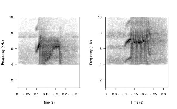
We can double-check that the bandpass actually worked by looking again at the spectrograms:
# extract the same 2 clips again
w1 <- read_wave(lbh.est, 12, from = 0, to = Inf)
w2 <- read_wave(lbh.est, 20, from = 0, to = Inf)

# split graphic device
par(mfrow = c(1, 2))

# plot spectros
spectro(w1, wl = 300, ovlp = 95, flim = c(1, 10), scale = FALSE,
        grid = FALSE, palette = reverse.gray.colors.1,
        collevels = seq(-70, 0, 5))

spectro(w2, wl = 300, ovlp = 95, flim = c(1, 10), scale = FALSE,
        grid = FALSE, palette = reverse.gray.colors.1,
        collevels = seq(-70, 0, 5))

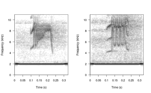
So any seewave function that works on ‘wave’ objects and returns ‘wave’ objects as well, can be used. For instance, applying a linear frequency shift to increase pitch in 2 kHz:
# load data
data("lbh.est")

# filter out freqs below 4 kHz
attributes(lbh.est)$wave.objects <- lapply(attributes(lbh.est)$wave.objects,
    FUN = lfs, shift = 2000, output = "Wave")

# extract the same 2 clips again
w1 <- read_wave(lbh.est, 12, from = 0, to = Inf)
w2 <- read_wave(lbh.est, 20, from = 0, to = Inf)

# split graphic device
par(mfrow = c(1, 2))

# plot spectros
spectro(w1, wl = 300, ovlp = 95, scale = FALSE,
        grid = FALSE, palette = reverse.gray.colors.1,
        collevels = seq(-70, 0, 5))

spectro(w2, wl = 300, ovlp = 95, scale = FALSE,
        grid = FALSE, palette = reverse.gray.colors.1,
        collevels = seq(-70, 0, 5))

Again, this should be OK as long as you don’t modify any time related feature. If temporal features change then the time annotations are no longer useful.
Session information
## R version 3.6.1 (2019-07-05)
## Platform: x86_64-pc-linux-gnu (64-bit)
## Running under: Ubuntu 18.04.4 LTS
##
## Matrix products: default
## BLAS:   /usr/lib/x86_64-linux-gnu/atlas/libblas.so.3.10.3
## LAPACK: /usr/lib/x86_64-linux-gnu/atlas/liblapack.so.3.10.3
##
## locale:
##  [1] LC_CTYPE=es_ES.UTF-8
##  [2] LC_NUMERIC=C
##  [3] LC_TIME=es_CR.UTF-8
##  [4] LC_COLLATE=es_ES.UTF-8
##  [5] LC_MONETARY=es_CR.UTF-8
##  [6] LC_MESSAGES=es_ES.UTF-8
##  [7] LC_PAPER=es_CR.UTF-8
##  [8] LC_NAME=C
##  [9] LC_ADDRESS=C
## [10] LC_TELEPHONE=C
## [11] LC_MEASUREMENT=es_CR.UTF-8
## [12] LC_IDENTIFICATION=C
##
## attached base packages:
## [1] stats     graphics  grDevices utils
## [5] datasets  methods   base
##
## other attached packages:
## [1] warbleR_1.1.24     seewave_2.1.5
## [3] tuneR_1.3.3        NatureSounds_1.0.3
## [5] knitr_1.28
##
## loaded via a namespace (and not attached):
##  [1] Rcpp_1.0.4.6    dtw_1.21-3
##  [3] fftw_1.0-6      digest_0.6.25
##  [5] bitops_1.0-6    MASS_7.3-51.4
##  [7] magrittr_1.5    signal_0.7-6
##  [9] evaluate_0.14   highr_0.8
## [11] rlang_0.4.6     stringi_1.4.6
## [13] pbapply_1.4-2   rmarkdown_1.17
## [15] rjson_0.2.20    tools_3.6.1
## [17] stringr_1.4.0   RCurl_1.98-1.2
## [19] proxy_0.4-24    xfun_0.13
## [21] yaml_2.2.1      parallel_3.6.1
## [23] compiler_3.6.1  htmltools_0.4.0