Some recent additions to warbleR aim to simplify the automatic detection of signals. The current post details these additions with a study case detecting inquiry calls of Spix’s disc-winged bats (Thyroptera tricolor).
Inquiry calls were recorded while the bats were flying in a flight cage. Recordings were made on four channels, each one from a different mic. Mics were about 1m apart from each other. So the four channels from a recording event represent slightly different registers of the same calls. This is an important characteristic of the data that will be taken into account in the analysis. Recordings were made as part of an ongoing study on indvidual variation in vocal activity at the Chaverri Lab.
To run this post you will need warbleR 1.1.24 (currently as the developmental version on github). It can be installed like this:
# From github
devtools::install_github("maRce10/warbleR")

# load warbleR
library(warbleR)
Recordings of Spix’s disc-winged bat inquiry calls can be downloaded like this:
# set temporary directory
setwd(tempdir())

# ids of figshare files to download
ids <- c(22496621, 22496585, 22495355, 22495397, 22473986, 22474022,
         22474586, 22474628)

nms <- c("1_ch2.wav", "2_ch2.wav", "2_ch1.wav", "1_ch1.wav", "1_ch4.wav",
         "2_ch4.wav", "1_ch3.wav", "2_ch3.wav")

for(i in 1:length(ids))
 download.file(url = paste0("https://ndownloader.figshare.com/files/", ids[i]),
 destfile = nms[i])
Cross-correlation based detection
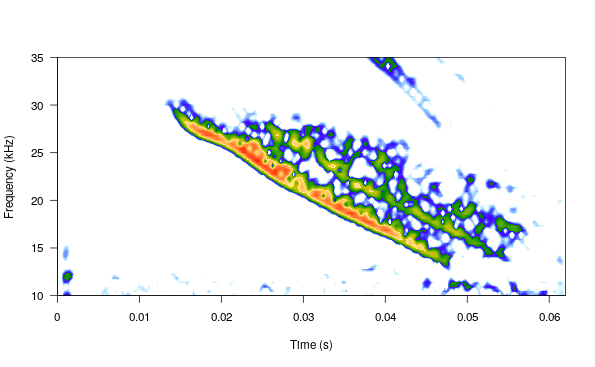
Cross-correlation can be used to detect highly stereotyped signals like the inquiry calls of Spix’s disc-winged bats. Cross-correlation detection uses an acoustic template to find similar signals across sound files. Hence, the first step is creating a template, which can be easily done by making a selection table with the time location of an example inquiry call (location was determined by scrolling over the spectrogram using Audacity):
# get a call template
templt <- data.frame(sound.files = "2_ch2.wav", selec = 2, channel = 1,
        start = 33.720, end = 33.756, stringsAsFactors = FALSE)

# read template as wave object
wv <- read_wave(templt, from = templt$start - 0.02, to = templt$end + 0.02)

# plot
spectro(wv, wl = 300, ovlp = 80, scale = FALSE, osc = FALSE, flim = c(10, 35),
        noisereduction = TRUE, grid = FALSE)
The second step requires making a selection table containing both the sound files in which to look for the template and the template itself:
# whole recordings selection table
sel_tab_1 <- selection_table(whole.recs = TRUE)
## all selections are OK
# add template selection
sel_tab <- rbind(templt, as.data.frame(sel_tab_1))

sel_tab
##   sound.files selec channel start      end
## 1   2_ch2.wav     2       1 33.72 33.75600
## 2   1_ch1.wav     1       1  0.00 48.88986
## 3   1_ch2.wav     1       1  0.00 48.88986
## 4   1_ch3.wav     1       1  0.00 48.88986
## 5   1_ch4.wav     1       1  0.00 48.88986
## 6   2_ch1.wav     1       1  0.00 49.54521
## 7   2_ch2.wav     1       1  0.00 49.54521
## 8   2_ch3.wav     1       1  0.00 49.54521
## 9   2_ch4.wav     1       1  0.00 49.54521
Finally, we must tell R which selection will be used as templates and where to look for them. To do this we need a two column matrix to indicate which selections should be used as templates (first column) and on which selections (or sound files) they will be detected (second column). If the name includes the selection number (‘selec’ column added at the end of the sound file name, e.g. “2_ch2.wav-2”) only the sound file segment specified in the selection will be used. If only the sound file name is included the function will look for the template across the entire sound file. In this case we want to use the first selection as template and run it over the entire sound files in ‘sel_tab’:
# pairwise comparison matrix
comp_mat <- cbind(paste(sel_tab$sound.files[1],
                        sel_tab$selec[1], sep = "-"), sel_tab$sound.files)

# look at it
comp_mat
##       [,1]          [,2]
##  [1,] "2_ch2.wav-2" "2_ch2.wav"
##  [2,] "2_ch2.wav-2" "1_ch1.wav"
##  [3,] "2_ch2.wav-2" "1_ch2.wav"
##  [4,] "2_ch2.wav-2" "1_ch3.wav"
##  [5,] "2_ch2.wav-2" "1_ch4.wav"
##  [6,] "2_ch2.wav-2" "2_ch1.wav"
##  [7,] "2_ch2.wav-2" "2_ch2.wav"
##  [8,] "2_ch2.wav-2" "2_ch3.wav"
##  [9,] "2_ch2.wav-2" "2_ch4.wav"
We are ready to detect signals using cross-correlation. In this example we use Mel-frequency cepstral coefficient cross-correlation (argument type = "mfcc"), which seems to work fine on these signals and tends to run faster than the more traditional Fourier transform spectrogram cross-correlation approach (but feel free to try it: type = "spcc"):
# run cross-correlation
xc_output <- xcorr(X = sel_tab, output = "list",
    compare.matrix = comp_mat, bp = c(12, 42), type = "mfcc", na.rm = TRUE)
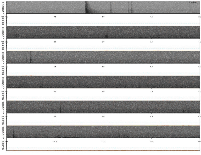
Note that the output was set to “list”, which includes a data frame with correlation scores by time for all sound files. This can be directly input into lspec() to visually explore the accuracy of the detection. The function lspec() plots the spectrogram of entire sound files split into multiple rows. However, if the output of xcorr() (or find_peaks(), see below) is supplied the function also plots a correlation score contour row below the spectrograms:
# plot
lspec(xc_output, sxrow = 2, rows = 6, flim = c(10, 50), fast.spec = TRUE,
      res = 60, horizontal = TRUE)
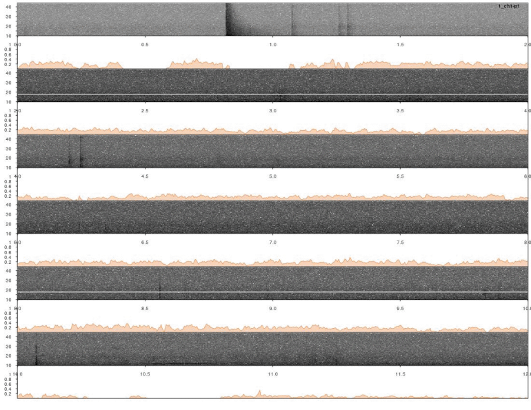
In this case a good detection routine should produce peaks in the score countour in the places where the inquiry calls are found. So it looks like it worked.
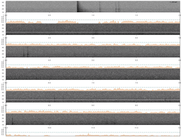
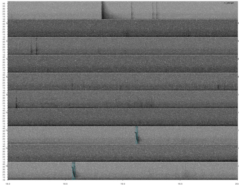
The output from xcorr() can also be taken by the function find_peaks() to detect signals. This function finds all instances in which the correlation scores goes above a certain threshold (‘cutoff’ argument, within 0-1 range). In this case a threshold of 0.4 seems to work well:
pks <- find_peaks(xc.output = xc_output, cutoff = 0.4, output = "list")
Again, if we used output= "list" in find_peaks(), the output can be plotted by lspec():
# plot
lspec(pks, sxrow = 2, rows = 6, flim = c(10, 50), fast.spec = TRUE,
      res = 60, horizontal = TRUE)
Detections look fine. However, we ran the analysis on all four channels for each sound file. So it’s very likely that some signals were detected more than once. We need to remove those duplicates. We can use the function ovlp_sels()to find them:
# extract selection table from find_peaks output
dup_peaks <- pks$selection.table

# rename sound files column so all channels belonging to the
# same sound file have the same sound file name momentarily
dup_peaks$org.sound.files <- dup_peaks$sound.files
dup_peaks$sound.files <- gsub("_ch[[:digit:]]", "", dup_peaks$sound.files)

# get overlapping sels
dup_peaks <- ovlp_sels(X = dup_peaks)

# get original sound files names back
dup_peaks$sound.files <- dup_peaks$org.sound.files
The function tags all overlapping selections with a unique label found in the column ‘ovlp.sels’ (last column):
dup_peaks
Now we just need to choose the selection with the highest cross-correlation score (‘dup_peaks$score’) for each group of overlapping selections:
# find highest score selection
detections <- dup_peaks[ave(x = dup_peaks$score, dup_peaks$ovlp.sels,
    FUN = function(x) rank(x, ties.method = "first")) == 1, ]
We can look again at the remaining detections. Now we are not intersted in detetions for individual channels but rather for each of the two recording event. So we can just plot all detections on the first channel for each sound file. To do this we must modify the sound file name like this:
# change channel to 1
detections$sound.files <- gsub("ch[[:digit:]]", "ch1", detections$sound.files)

# plot
lspec(detections, sxrow = 2, rows = 6, flim = c(10, 50),
      fast.spec = TRUE, res = 60, horizontal = TRUE)
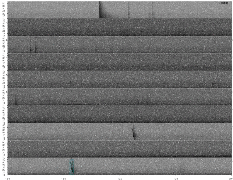
Overall it looks OK, but some signals were not detected. This could be fixed by decreasing the correlation threshold. Alternatively, we could use several templates that better represent the variation in call structure. If taking the second approach, the same trick can be used for excluding duplicated detections (removing overlapping detections using ovlp_sels()).
Amplitude threshold based detection
Amplitude detectors can be an useful alternative to cross-correlation. These detectors don’t require highly stereotyped signals, although they work better on high quality recordings in which the amplitude of target signals is higher than background noise (i.e. high signal-to-noise ratio). The function auto_detec() performs this type of detection. In this case we use the initial selection table to detect inquiry calls. The first 1.5 s of the recordings are excluded to get rid of a very loud clap at the beginning of sound files:
# remove clap
sel_tab_1$start <- 1.5

# detect
ad <- auto_detec(X = sel_tab_1, threshold = 30, ssmooth = 700, mindur = 0.005, wl = 1000,
        maxdur = 0.05, bp = c(10, 50), output = "list", img = FALSE)
Note that we also used time filters (‘mindur’ and ‘maxdur’) and a bandpass filter (‘bp’). This are set based on our previous knowledge of the target signal duration and frequency range. The argument output = "list" generates an R object that can be taken by lspec(), similarly as in previous examples. This is how the detection looks like:
# plot
lspec(ad, sxrow = 2, flim = c(10, 50), rows = 6,
      fast.spec = TRUE, res = 60, horizontal = TRUE)
Again, we need to remove duplicated detection. In this case there are no correlation scores so we just simply find the overlapping detections and remove the duplicated ones:
# extract selection table from find_peaks output
dup_ad <- ad$selection.table

# rename sound files column so all channels belonging to the
# same sound file have the same sound file name momentarily
dup_ad$org.sound.files <- dup_ad$sound.files
dup_ad$sound.files <- gsub("_ch[[:digit:]]", "", dup_ad$sound.files)

# get overlapping sels
dup_ad <- ovlp_sels(X = dup_ad)

# remove duplicaets
ad_detections <- dup_ad[!duplicated(dup_ad$ovlp.sels, incomparables = NA), ]

# get original sound files names back
ad_detections$sound.files <- ad_detections$org.sound.files
We can now look at the remaining detections. We need to modify the sound file name so they are all plotted on the first channel:
# change channel to 1
ad_detections$sound.files <- gsub("ch[[:digit:]]", "ch1", ad_detections$sound.files)

# plot
lspec(ad_detections, sxrow = 2, rows = 10, flim = c(10, 50),
      fast.spec = TRUE, res = 60, horizontal = TRUE)
Most calls were detected but not all of them. This detection could improve by adjusting the detection parameters (i.e. ’threshold’, ‘ssmooth’, etc). Nonetheless, the example is good enough to show how to do these analyses in R.
Session information
## R version 3.6.1 (2019-07-05)
## Platform: x86_64-pc-linux-gnu (64-bit)
## Running under: Ubuntu 18.04.4 LTS
##
## Matrix products: default
## BLAS:   /usr/lib/x86_64-linux-gnu/atlas/libblas.so.3.10.3
## LAPACK: /usr/lib/x86_64-linux-gnu/atlas/liblapack.so.3.10.3
##
## locale:
##  [1] LC_CTYPE=es_ES.UTF-8       LC_NUMERIC=C
##  [3] LC_TIME=es_CR.UTF-8        LC_COLLATE=es_ES.UTF-8
##  [5] LC_MONETARY=es_CR.UTF-8    LC_MESSAGES=es_ES.UTF-8
##  [7] LC_PAPER=es_CR.UTF-8       LC_NAME=C
##  [9] LC_ADDRESS=C               LC_TELEPHONE=C
## [11] LC_MEASUREMENT=es_CR.UTF-8 LC_IDENTIFICATION=C
##
## attached base packages:
## [1] stats     graphics  grDevices utils     datasets
## [6] methods   base
##
## other attached packages:
## [1] kableExtra_1.1.0   warbleR_1.1.24     NatureSounds_1.0.3
## [4] seewave_2.1.6      tuneR_1.3.3        knitr_1.28
##
## loaded via a namespace (and not attached):
##  [1] Rcpp_1.0.4.6      highr_0.8         compiler_3.6.1
##  [4] pillar_1.4.4      bitops_1.0-6      tools_3.6.1
##  [7] digest_0.6.25     viridisLite_0.3.0 evaluate_0.14
## [10] tibble_3.0.1      lifecycle_0.2.0   fftw_1.0-6
## [13] pkgconfig_2.0.3   rlang_0.4.6       rstudioapi_0.11
## [16] yaml_2.2.1        parallel_3.6.1    xfun_0.14
## [19] xml2_1.3.2        stringr_1.4.0     httr_1.4.1
## [22] vctrs_0.3.1       hms_0.5.3         webshot_0.5.2
## [25] glue_1.4.1        R6_2.4.1          dtw_1.21-3
## [28] pbapply_1.4-2     rmarkdown_2.2     readr_1.3.1
## [31] magrittr_1.5      scales_1.1.1      htmltools_0.4.0
## [34] ellipsis_0.3.1    MASS_7.3-51.4     rvest_0.3.5
## [37] colorspace_1.4-1  stringi_1.4.6     proxy_0.4-24
## [40] munsell_0.5.0     signal_0.7-6      RCurl_1.98-1.2
## [43] crayon_1.3.4      rjson_0.2.20