Provide tools for double-checking the quality of the acoustic data and measures
When working with sound files obtained from various sources it is common to have variation in recording formats and parameters or even find corrupt files. Similarly, when a large number of annotations are used, it is normal to find errors in some of them. These problems may prevent the use of acoustic analysis in warbleR. Luckily, the package also offers functions to facilitate the detection and correction of errors in sound files and annotations.
1 Organize acoustic data
1.1 Consolidate files
The consolidate() function allows you to copy all the sound files in a specified format (e.g. ‘.wav’) from subdirectories into a single directory. This is useful when you have sound files in different folders and want to analyze them together using warbleR. The function creates a new folder called ‘consolidated_files’ in the working directory and copies all the files with the specified extension into it. Let’s see how it works with the example files in the ‘./examples’ folder:
The output is a data frame with the original paths and the original and new file names. Note that if there are files with the same name in different folders, the function adds a number to the end of the file name to avoid overwriting. It also labels possible duplicates in the output data frame.
2 Homogenize recording format
2.1 Convert .mp3 to .wav
The mp32wav() function allows you to convert files in ‘.mp3’ format to ‘.wav’ format. This function converts all the ‘mp3’ files in the working directory. Let’s use the files in the ‘./examples/mp3’ folder as an example. This are the ‘mp3’ files in that folder:
We can check the properties of the sound files using the info_sound_files() function:
Code
info_sound_files(path ="./examples/mp3")
sound.files
duration
sample.rate
channels
bits
wav.size
samples
BlackCappedVireo.mp3
5.459592
22.05
1
16
0.087770
120384
BlackCappedVireo.wav
5.459592
22.05
1
16
0.240812
120384
BowheadWhaleSong.mp3
86.648163
22.05
1
16
1.386787
1910592
BowheadWhaleSong.wav
86.648163
22.05
1
16
3.821228
1910592
CanyonWren.mp3
5.433469
44.10
1
16
0.087352
239616
CanyonWren.wav
5.433469
44.10
1
16
0.479276
239616
2.2 Homogenize .wav files
Alternatively, we can use the fix_wavs() function to homogenize the sampling rate, the dynamic interval and the number of channels. It is adviced that all sound files should have the same recording format settings before any acoustic analysis. In the example ‘.mp3’ files, not all of them have been recorded with the same settings:
Code
info_sound_files(path ="./examples/mp3")
sound.files
duration
sample.rate
channels
bits
wav.size
samples
BlackCappedVireo.mp3
5.459592
22.05
1
16
0.087770
120384
BlackCappedVireo.wav
5.459592
22.05
1
16
0.240812
120384
BowheadWhaleSong.mp3
86.648163
22.05
1
16
1.386787
1910592
BowheadWhaleSong.wav
86.648163
22.05
1
16
3.821228
1910592
CanyonWren.mp3
5.433469
44.10
1
16
0.087352
239616
CanyonWren.wav
5.433469
44.10
1
16
0.479276
239616
The fix_wavs() function will convert all files to the same sampling rate and dynamic range:
The resample_est()` function allows you to homogenize sampling rate and dynamic range of an extended selection table. This is useful when the selection table contains selections from recordings with different sampling rates or dynamic ranges. Let’s see how it works with the example ‘lbh.ext’ selection table. First check the sampling rates and bit depths of the acoustic data in the selection table:
Code
data("lbh.est")# check sampling rates and bit depthsunique(attributes(lbh.est)$check.res$sample.rate)
[1] 22.05
Code
unique(attributes(lbh.est)$check.res$bits)
[1] "8"
Now let’s resample the recordings to a sampling rate of 11.025 kHz and a bit depth of 24:
Code
lbh.est_resamp <-resample_est(X = lbh.est,samp.rate =11.025,bit.depth =24)# check sampling rates and bit depths againunique(attributes(lbh.est_resamp)$check.res$sample.rate)
[1] 11.025
Code
unique(attributes(lbh.est_resamp)$check.res$bits)
[1] "24"
3 Check recordings
check_sound_files() should be the first function that should be used before running any warbleR analysis. The function simply checks if the sound files in ‘.wav’ format in the working directory can be read in R. For example, the following code checks all the files in the ‘examples’ folder, which should detect the ‘corrupted_file.wav’:
Code
check_sound_files(path ="./examples")
All files can be read
Not all sound files have the same sampling rate (potentially problematic, particularly for cross_correlation())
Let’s see how it works when we simulate a corrupted file:
Code
# save text file as wave filewriteLines("This is not a wave file", con ="./examples/corrupted_file.wav")# check againchecks <-check_sound_files(path ="./examples")checks
sound.files
samp.rate
result
bit24.wav
44100
can be read
bit64.wav
44100
can be read
bit8.wav
44100
can be read
corrupted_file.wav
NA
cannot be read
downsmp.wav
11250
can be read
LBH.374.SUR.wav
44100
can be read
Phae.long1.flac
22050
can be read
Phae.long1.mp3
22050
can be read
Phae.long1.wav
22500
can be read
Phae.long2.wav
22500
can be read
Phae.long3.wav
22500
can be read
Phae.long4.wav
22500
can be read
Phaethornis-eurynome-15607.wav
44100
can be read
Phaethornis-squalidus-555876.mp3
48000
can be read
Phaethornis-striigularis-154074.mp3
44100
can be read
Phaethornis-striigularis-518510.mp3
48000
can be read
Phaethornis-striigularis-537364.mp3
44100
can be read
recording_20170716_230503.wac
384000
can be read
song.dynrang.wav
44100
can be read
song.dynrang24.wav
44100
can be read
test.wav
11025
can be read
4 Optimizing spectrograms
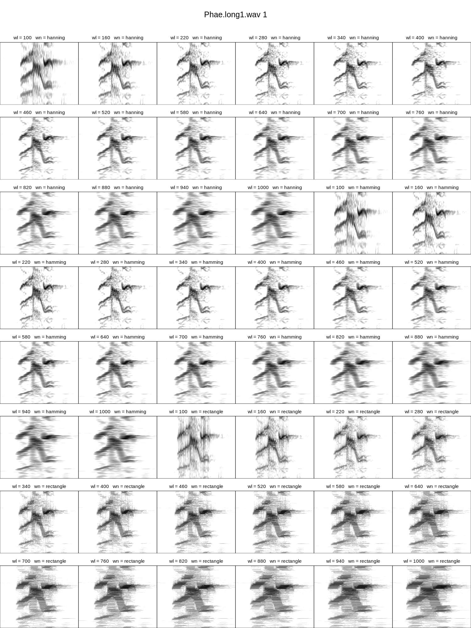
The parameters that determine the appearance of spectrograms (and power spectra and periodgrams) also have an effect on the measurements taken on them. Therefore it is necessary to use the same parameters to analyze all the signals in a project (except with some exceptions) so that the measurements are comparable. The visualization of spectrograms generated with different spectrographic parameters is a useful way of defining the combination of parameters with which the structure of the signals is distinguished in more detail. The function tweak_spectro() aims to simplify the selection of parameters through the display of spectrograms. The function plots, for a single selection, a mosaic of spectrograms with different display parameters. For numerical arguments, the upper and lower limits of a range can be provided. The following parameters may have variable values:
wl: window length (numerical range)
ovlp: overlap (numerical range)
collev.min: minimum amplitude value for color levels (numerical range)
wn: window function name (character)
pal: palette (character)
The following code generates an image with spectrograms that vary in window size and window function (the rest of the parameters are passed to the catalog () function internally to create the mosaic):
Note that the length.out argument defines the number of values to interpolate within the numerical ranges. wl = 220 seems to produce clearer spectrograms.
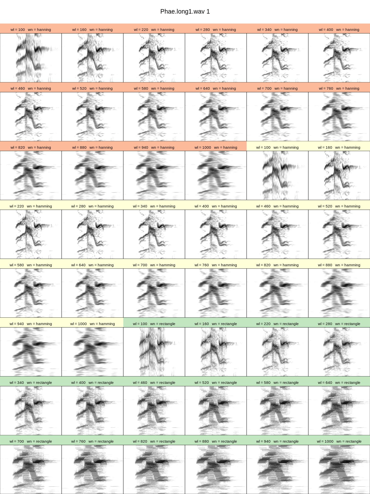
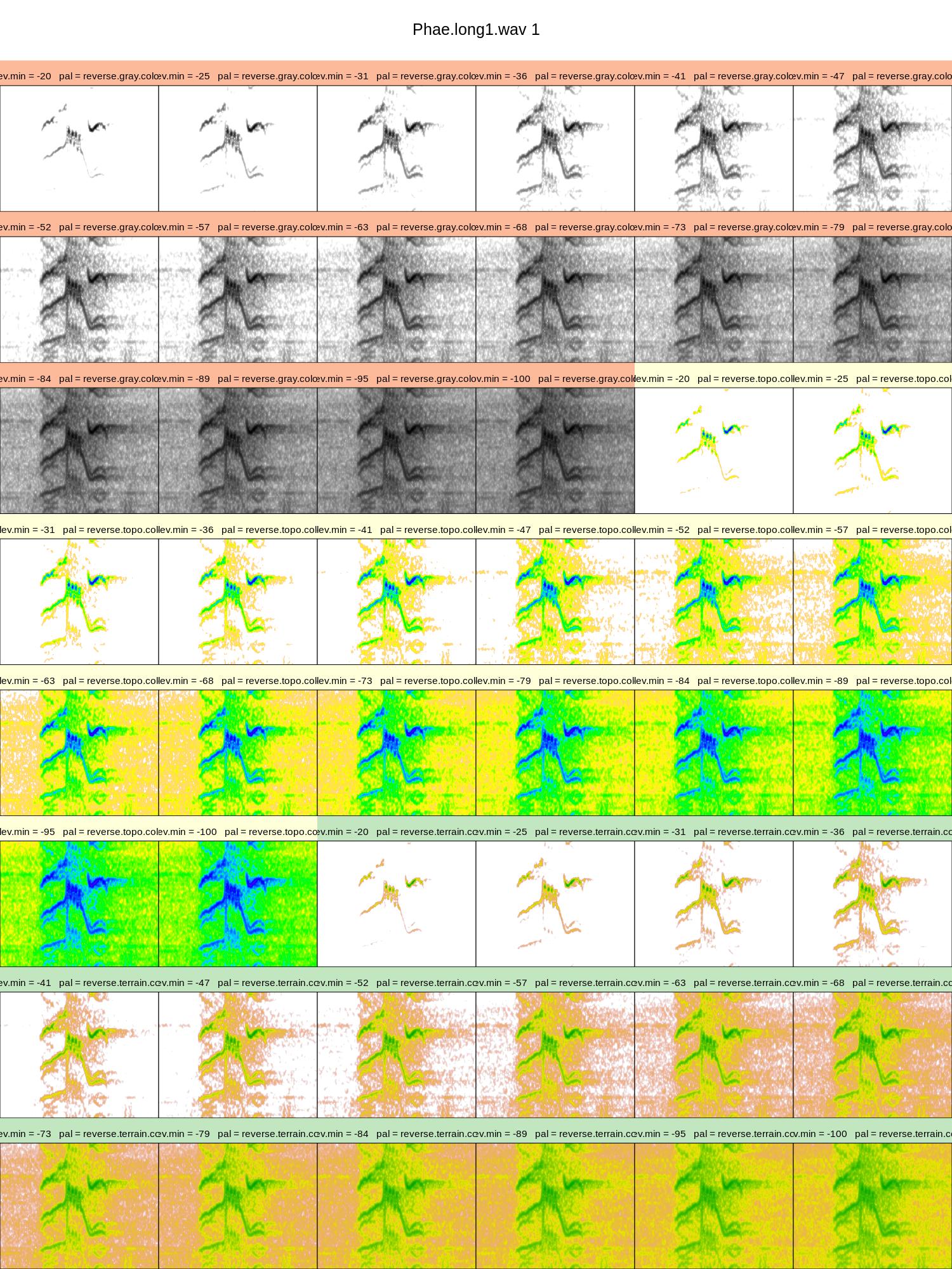
We can add a color palette to differentiate the levels of one of the parameters, for example ‘wn’:
The file iniquiry_calls.RDS (in ./examples) contains an extended selection table of inquiry calls of Spix’s disc-winged bats (Thyroptera tricolor). This is a Neotropical species that uses a specific call type to locate social mates in their roosts. We can read this file like this:
Using the ‘inq’ data, find the best window length (‘wl’) to visualize the inquiry calls using tweak_spectro() (keep in mind this are ultrasonic signals)
Try 3 color palettes from the package ‘viridis’ to visualize the spectrograms (you will need to install and load the package) while also testing different collev.min values.
5 Double-check selections
The main function to double-check selection tables is check_sels(). This function checks a large number of possible errors in the selection information:
‘X’ is an object of the class ‘data.frame’ or ‘selection_table’ (see selection_table) and contains the columns required to be used in any warbleR function (‘sound.files’, ‘selec’, ‘start’ , ‘end’, if it does not return an error)
‘sound.files’ in ‘X’ corresponds to the .wav files in the working directory or in the provided ‘path’ (if no file is found it returns an error, if some files are not found it returns error information in the output data frame)
the time (‘start’, ‘end’) and frequency limits (‘bottom.freq’, ‘top.freq’, if provided) are numeric and do not contain NA (if they do not return an error)
There are no duplicate selection tags (‘selec’) within a sound file (if it does not return an error)
The start and end time of the selections is within the duration of the sound files (error information in the output data frame)
Sound files can be read (error information in the output data frame)
The header of the sound files is not damaged (only if the header = TRUE, error information in the selection table with results)
‘top.freq’ is less than half of the sampling frequency (nyquist frequency, error information in the data table with results)
Negative values are not found in the time or frequency limits (error information in the data table with results)
‘start’ higher than ‘end’ or ‘bottom.freq’ higher than ‘top.freq’ (error information in the output data frame)
The value of ‘channel’ is not greater than the number of channels in the sound files (error information in the output data frame)
Code
cs <-check_sels(lbh_selec_table)
The function returns a data frame that includes the information in ‘X’ plus additional columns about the format of the sound files, as well as the result of the checks (column ‘check.res’):
Code
cs
sound.files
channel
selec
start
end
bottom.freq
top.freq
check.res
duration
min.n.samples
sample.rate
channels
bits
sound.file.samples
Phae.long1.wav
1
1
1.1693549
1.3423884
2.220105
8.604378
OK
0.1730334
3893
22.5
1
16
56251
Phae.long1.wav
1
2
2.1584085
2.3214565
2.169437
8.807053
OK
0.1630480
3668
22.5
1
16
56251
Phae.long1.wav
1
3
0.3433366
0.5182553
2.218294
8.756604
OK
0.1749187
3935
22.5
1
16
56251
Phae.long2.wav
1
1
0.1595983
0.2921692
2.316862
8.822316
OK
0.1325709
2982
22.5
1
16
38251
Phae.long2.wav
1
2
1.4570585
1.5832087
2.284006
8.888027
OK
0.1261502
2838
22.5
1
16
38251
Phae.long3.wav
1
1
0.6265520
0.7577715
3.006834
8.822316
OK
0.1312195
2952
22.5
1
16
49500
Phae.long3.wav
1
2
1.9742132
2.1043921
2.776843
8.888027
OK
0.1301789
2929
22.5
1
16
49500
Phae.long3.wav
1
3
0.1233643
0.2545812
2.316862
9.315153
OK
0.1312170
2952
22.5
1
16
49500
Phae.long4.wav
1
1
1.5168116
1.6622365
2.513997
9.216586
OK
0.1454249
3272
22.5
1
16
72000
Phae.long4.wav
1
2
2.9326920
3.0768784
2.579708
10.235116
OK
0.1441864
3244
22.5
1
16
72000
Phae.long4.wav
1
3
0.1453977
0.2904966
2.579708
9.742279
OK
0.1450989
3264
22.5
1
16
72000
Let’s modified a selection table to see how the function works:
Code
# copiar las primeras 6 filasst2 <- lbh_selec_table[1:6, ]# hacer caracter st2$sound.files <-as.character(st2$sound.files)# cambiar nombre de archivo de sonido en sel 1st2$sound.files[1] <-"aaa.wav"# modificar fin en sel 3st2$end[3] <-100# hacer top.freq igual q bottom freq en sel 3st2$top.freq[3] <- st2$bottom.freq[3]# modificar top freq en sel 5st2$top.freq[5] <-200# modificar channes en sel 6st2$channel[6] <-3#revisarcs <-check_sels(st2)cs[, c(1:7, 10)]
sound.files
channel
selec
start
end
bottom.freq
top.freq
min.n.samples
aaa.wav
1
1
1.1693549
1.3423884
2.220105
8.604378
NA
Phae.long1.wav
1
2
2.1584085
2.3214565
2.169437
8.807053
3668
Phae.long1.wav
1
3
0.3433366
100.0000000
2.218294
2.218294
2242274
Phae.long2.wav
1
1
0.1595983
0.2921692
2.316862
8.822316
2982
Phae.long2.wav
1
2
1.4570585
1.5832087
2.284006
200.000000
2838
Phae.long3.wav
1
1
0.6265520
0.7577715
3.006834
8.822316
2952
check_sels() is used internally when creating selection tables and extended selection tables.
5.0.1 Visual inspection of spectrograms
Once the information in the selections has been verified, the next step is to ensure that the selections contain accurate information about the location of the signals of interest. This can be done by creating spectrograms of all selections. For this we have several options. The first is spectrograms() (previously called specreator()) which generates (by default) a spectrogram for each selection. We can run it on the sample data like this:
The images it produces are saved in the working directory and look like this:
Exercise
Have the label shown on the selection display the data in the ‘sel.comment’ column of the sample selection box using the sel.labels argument
5.0.2 Full spectrograms
We can create spectrograms for the whole sound files using full_spectrograms(). If the X argument is not given, the function will create the spectrograms for all the files in the working directory. Otherwise, the function generates spectrograms for sound files in X and highlights selections with transparent rectangles similar to those ofspectrograms(). In this example we download a recording from a striped-throated hermit (Phaethornis striigularis) from Xeno-Canto:
Code
# load package with color paletteslibrary(viridis)# create directorydir.create("./examples/hermit")# download sound filephae.stri <-query_xc(qword ="nr:154074",download =TRUE,path ="./examples/hermit")# Convert mp3 to wav formatmp32wav(path ="./examples/hermit/", pb =FALSE)# plot full specfull_spectrograms(sxrow =1,rows =10,pal = magma,wl =200,flim =c(3, 10),collevels =seq(-140, 0, 5),path ="./examples/hermit/")
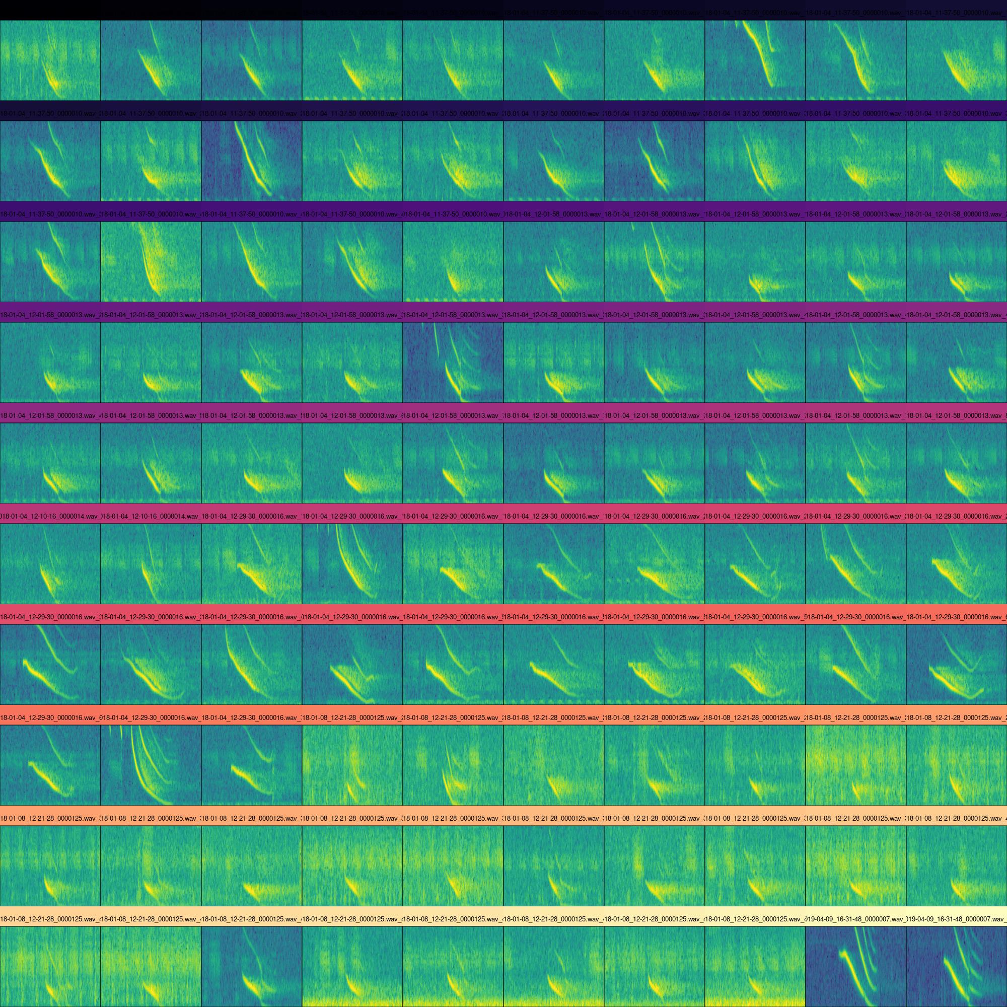
5.1 Catalogs
Catalogs allow you to inspect selections of many recordings in the same image and group them by categories. This makes it easier to verify the consistency of the categories. Many of the arguments are shared with tweak_spectro() (catalog() is used internally in tweak_spectro()). We can generate a catalog with color tags to identify selections from the same sound file as follows:
- Modify the previous code of catalog() to create a catalog with 5 rows and 20 columns, using the ‘wl’ value and color palette that you considered best when using tweak_spectro() with the ‘inq’ data.
Using the ‘lbh_selec_table’ data, create a catalog with selections color-tagged by song type
5.2 Tailoring selections
The position of the selections in the sound file (i.e. its ‘coordinates’ of time and frequency) can be modified interactively from R using the sel_tailor() function. This function produces a graphic window showing spectrograms and a series of ‘buttons’ that allow you to modify the view and move forward in the selection table: