R basics

Tropical Biology 2022
Organization for Tropical Studies

---

What is R?

• A free Domain-Specific-Language (DSL) for statistics and data analysis
• A collection of over 18949 (mar-9-2022) libraries
• A large and active community across industry and academia
• A way to talk “directly” to your computer

Historically:

• Based on the S Programming Language
• Around 20 years old (Lineage dates from 1975 - almost 40 years ago)

 

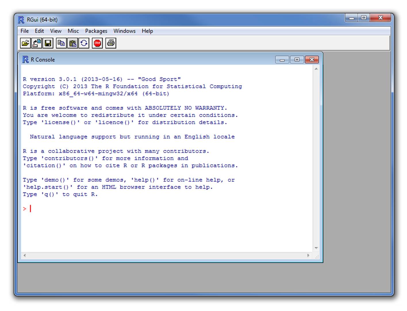
Rstudio

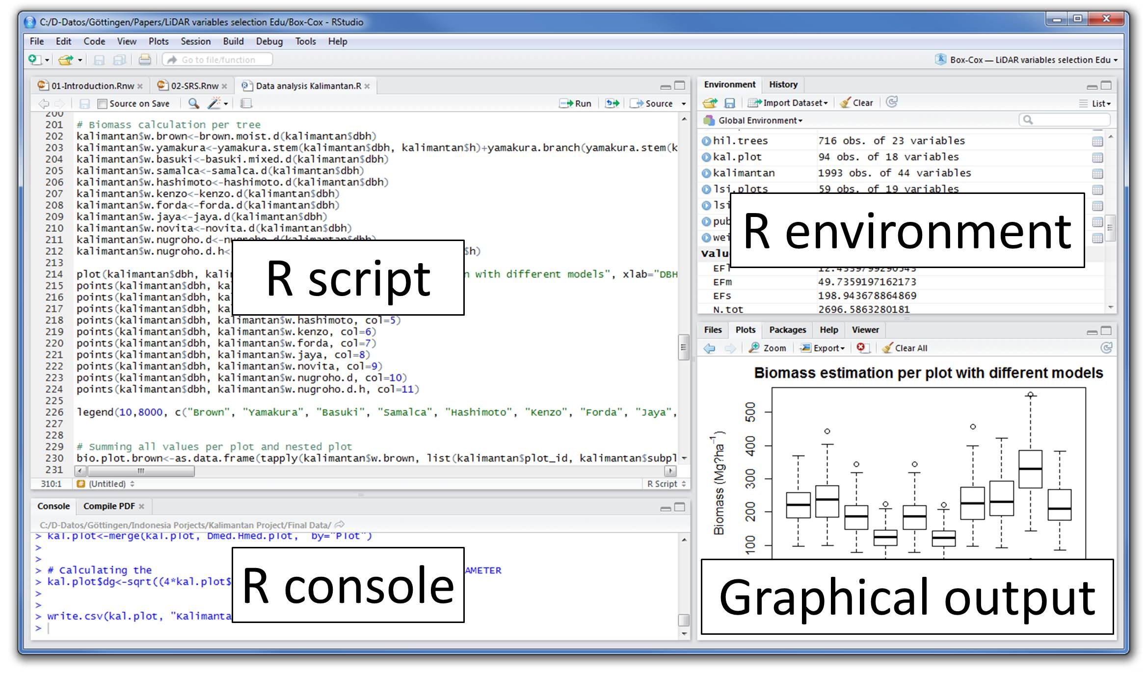
Integrated development environment (IDE) for R. Includes:

• A console
• Syntax-highlighting editor that supports direct code execution
• Tools for plotting, history, debugging and workspace management

---

Elements of the R language

• Vectors
• Lists
• Matrices
• Data Frames
• Tables
• Functions (including operators)
• Attributes
• Arrays
• Environments

Data structure

The basic data structure in R is the vector. There are two basic types of vectors: atomic vectors and lists.

They have three common properties:

• Type, typeof() (~ class/mode)
• Length, length() (number of elements)
• Attributes, attributes() (metadata)

They differ in the types of their elements: all elements of an atomic vector must be the same type, whereas the elements of a list can have different types.

	Homogeneous	Heterogeneous
1d	Atomic vector	List
2d	Matrix	Data frame
nd	Array

 

R has no 0-dimensional elements (scalars). Individual numbers or strings are actually vectors of length one.

Atomic vectors

Types of atomic vectors:

• Logical (boolean)
• Integer
• Numeric (double)
• Character

Vectors are built using c():

x <- 1
x1 <- c(1)

all.equal(x, x1)
## [1] TRUE

class(x)
## [1] "numeric"

y <- "something"

class(y)
## [1] "character"

w <- 1L

class(w)
## [1] "integer"
 
z <- TRUE

class(z)
## [1] "logical"

q <- factor(1)

class(q)
## [1] "factor"

 

Vectors can only contain entries of the same type. Different types will be coerced to the most flexible type:

v <- c(10, 11, 12, 13)

class(v)
## [1] "numeric"

typeof(v)
## [1] "double"

is.integer(v)
## [1] FALSE

y <- c("Amazona", "Ara", "Eupsittula", "Myiopsitta")

class(y)
## [1] "character"

is.integer(y)
## [1] FALSE

x <- c(1,2,3, "Myiopsitta")

x
## [1] "1"          "2"          "3"          "Myiopsitta"

class(x)
## [1] "character"

 

Missing values are specified with NA, which is a logical vector of length 1. NA will always be coerced to the correct type if used inside c():

v <- c(10, 11, 12, 13, NA)

class(v)
## [1] "numeric"

v <- c(letters[1:3], NA)

class(v)
## [1] "character"

 

Lists

Can contain objects of different classes and sizes. Lists are built using list():

l <- list(ID = c("a", "b", "c", "d", "e"), size = c(1, 2, 3, 4, 5), observed = c(FALSE, TRUE, FALSE, FALSE, FALSE))

l

## $ID
## [1] "a" "b" "c" "d" "e"
## 
## $size
## [1] 1 2 3 4 5
## 
## $observed
## [1] FALSE  TRUE FALSE FALSE FALSE

class(l)

## [1] "list"

str(l)

## List of 3
##  $ ID      : chr [1:5] "a" "b" "c" "d" ...
##  $ size    : num [1:5] 1 2 3 4 5
##  $ observed: logi [1:5] FALSE TRUE FALSE FALSE FALSE

… and dimensions:

l <- list(ID = c("a", "b", "c", "d", "e"), size = c(1, 2, 3, 4, 5, 6), observed = c(FALSE, TRUE, FALSE, FALSE, FALSE), l)

str(l)

## List of 4
##  $ ID      : chr [1:5] "a" "b" "c" "d" ...
##  $ size    : num [1:6] 1 2 3 4 5 6
##  $ observed: logi [1:5] FALSE TRUE FALSE FALSE FALSE
##  $         :List of 3
##   ..$ ID      : chr [1:5] "a" "b" "c" "d" ...
##   ..$ size    : num [1:5] 1 2 3 4 5
##   ..$ observed: logi [1:5] FALSE TRUE FALSE FALSE FALSE

l2 <- list(l, l)

str(l2)

## List of 2
##  $ :List of 4
##   ..$ ID      : chr [1:5] "a" "b" "c" "d" ...
##   ..$ size    : num [1:6] 1 2 3 4 5 6
##   ..$ observed: logi [1:5] FALSE TRUE FALSE FALSE FALSE
##   ..$         :List of 3
##   .. ..$ ID      : chr [1:5] "a" "b" "c" "d" ...
##   .. ..$ size    : num [1:5] 1 2 3 4 5
##   .. ..$ observed: logi [1:5] FALSE TRUE FALSE FALSE FALSE
##  $ :List of 4
##   ..$ ID      : chr [1:5] "a" "b" "c" "d" ...
##   ..$ size    : num [1:6] 1 2 3 4 5 6
##   ..$ observed: logi [1:5] FALSE TRUE FALSE FALSE FALSE
##   ..$         :List of 3
##   .. ..$ ID      : chr [1:5] "a" "b" "c" "d" ...
##   .. ..$ size    : num [1:5] 1 2 3 4 5
##   .. ..$ observed: logi [1:5] FALSE TRUE FALSE FALSE FALSE

 

Names

Vectors can be named in three ways:

• When creating it: x <- c(a = 1, b = 2, c = 3)
• By modifying an existing vector in place: x <- 1:3; names(x) <- c("a", "b", "c") Or: x <- 1:3; names(x)[[1]] <- c("a")
• By creating a modified copy of a vector: x <- setNames(1:3, c("a", "b", "c"))

y <- c(a = 1, 2, 3)

names(y)

## [1] "a" ""  ""

v <- c(1, 2, 3)

names(v) <- c('a')

names(v)

## [1] "a" NA  NA

z <- setNames(1:3, c("a", "b", "c"))

names(z)

## [1] "a" "b" "c"

 

Factors

Attributes are used to define factors. A factor is a vector that can contain only predefined values, and is used to store categorical data.

Factors are built on top of integer vectors using two attributes:

• class “factor”: makes them behave differently from regular integer vectors
• levels: defines the set of allowed values

x <- factor(c("a", "b", "b", "a"))
x

## [1] a b b a
## Levels: a b

levels(x)

## [1] "a" "b"

str(x)

##  Factor w/ 2 levels "a","b": 1 2 2 1

 

Factors look like character vectors but they are actually integers:

x <- factor(c("a", "b", "b", "a"))

c(x)

## [1] a b b a
## Levels: a b

 

Matrices

All entries are of the same type:

m <- matrix(c(1, 2, 3, 11, 12, 13), nrow = 2)

dim(m)

## [1] 2 3

m

##      [,1] [,2] [,3]
## [1,]    1    3   12
## [2,]    2   11   13

class(m)

## [1] "matrix" "array"

m <- matrix(c(1, 2, 3, 11, 12,"13"), nrow = 2)
m

##      [,1] [,2] [,3]
## [1,] "1"  "3"  "12"
## [2,] "2"  "11" "13"

 

Can be created by modifying the dimension attribute:

c <- 1:6

is.matrix(c)

## [1] FALSE

attributes(c)

## NULL

dim(c) <- c(3, 2)

c

##      [,1] [,2]
## [1,]    1    4
## [2,]    2    5
## [3,]    3    6

is.matrix(c)

## [1] TRUE

attributes(c)

## $dim
## [1] 3 2

 

Data frames

Special case of lists. Can contain entries of different types:

m <- data.frame(ID = c("a", "b", "c", "d", "e"), size = c(1, 2, 3, 4, 5), observed = c(FALSE, TRUE, FALSE, FALSE, FALSE))

dim(m)

## [1] 5 3

m

##   ID size observed
## 1  a    1    FALSE
## 2  b    2     TRUE
## 3  c    3    FALSE
## 4  d    4    FALSE
## 5  e    5    FALSE

class(m)

## [1] "data.frame"

is.data.frame(m)

## [1] TRUE

is.list(m)

## [1] TRUE

str(m)

## 'data.frame':    5 obs. of  3 variables:
##  $ ID      : chr  "a" "b" "c" "d" ...
##  $ size    : num  1 2 3 4 5
##  $ observed: logi  FALSE TRUE FALSE FALSE FALSE

 

But vectors should have the same length:

m <- data.frame(ID = c("a", "b", "c", "d", "e"), size = c(1, 2, 3, 4, 5, 6), observed = c(FALSE, TRUE, FALSE, FALSE, FALSE))

## Error in data.frame(ID = c("a", "b", "c", "d", "e"), size = c(1, 2, 3, : arguments imply differing number of rows: 5, 6

 

---

Data subsetting

Indexing

Elements within objects can be called by indexing. To subset a vector simply call the object position using square brackets:

x <- c(1, 3, 4, 10, 15, 20, 50, 1, 6)

x[1]

## [1] 1

x[2]

## [1] 3

x[2:3]

## [1] 3 4

x[c(1,3)]

## [1] 1 4

 

Elements can be removed in the same way:

x[-1]

## [1]  3  4 10 15 20 50  1  6

x[-c(1,3)]

## [1]  3 10 15 20 50  1  6

 

Matrices and data frames required 2 indices [row, column]:

m <- matrix(c(1, 2, 3, 11, 12, 13), nrow = 2)

m[1, ]

## [1]  1  3 12

m[, 1]

## [1] 1 2

m[1, 1]

## [1] 1

m[-1, ]

## [1]  2 11 13

m[, -1]

##      [,1] [,2]
## [1,]    3   12
## [2,]   11   13

m[-1, -1]

## [1] 11 13

df <- data.frame(family = c("Psittacidae", "Trochilidae", 
                            "Psittacidae"), 
  genus = c("Amazona", "Phaethornis", "Ara"), 
    species = c("aestiva", "philippii", "ararauna"))

df

##        family       genus   species
## 1 Psittacidae     Amazona   aestiva
## 2 Trochilidae Phaethornis philippii
## 3 Psittacidae         Ara  ararauna

df[1, ]

##        family   genus species
## 1 Psittacidae Amazona aestiva

df[, 1]

## [1] "Psittacidae" "Trochilidae" "Psittacidae"

df[1, 1]

## [1] "Psittacidae"

df[-1, ]

##        family       genus   species
## 2 Trochilidae Phaethornis philippii
## 3 Psittacidae         Ara  ararauna

df[, -1]

##         genus   species
## 1     Amazona   aestiva
## 2 Phaethornis philippii
## 3         Ara  ararauna

df[-1, -1]

##         genus   species
## 2 Phaethornis philippii
## 3         Ara  ararauna

df[,"family"]

## [1] "Psittacidae" "Trochilidae" "Psittacidae"

df[,c("family", "genus")]

##        family       genus
## 1 Psittacidae     Amazona
## 2 Trochilidae Phaethornis
## 3 Psittacidae         Ara

 

Lists require 1 index within double square brackets [[index]]:

l <- list(ID = c("a", "b", "c", "d", "e"), size = c(1, 2, 3, 4, 5), observed = c(FALSE, TRUE, FALSE, FALSE, FALSE))

l[[1]]

## [1] "a" "b" "c" "d" "e"

l[[3]]

## [1] FALSE  TRUE FALSE FALSE FALSE

 

Elements within lists can also be subset in the same string of code:

l[[1]][1:2]

## [1] "a" "b"

l[[3]][2]

## [1] TRUE

 

Exploring objects

str(df)

## 'data.frame':    3 obs. of  3 variables:
##  $ family : chr  "Psittacidae" "Trochilidae" "Psittacidae"
##  $ genus  : chr  "Amazona" "Phaethornis" "Ara"
##  $ species: chr  "aestiva" "philippii" "ararauna"

names(df)

## [1] "family"  "genus"   "species"

dim(df)

## [1] 3 3

nrow(df)

## [1] 3

ncol(df)

## [1] 3

head(df)

##        family       genus   species
## 1 Psittacidae     Amazona   aestiva
## 2 Trochilidae Phaethornis philippii
## 3 Psittacidae         Ara  ararauna

tail(df)

##        family       genus   species
## 1 Psittacidae     Amazona   aestiva
## 2 Trochilidae Phaethornis philippii
## 3 Psittacidae         Ara  ararauna

table(df$genus)

## 
##     Amazona         Ara Phaethornis 
##           1           1           1

typeof(df)

## [1] "list"

View(df)

 

Exercise

 

• Using the example data iris to create a data subset with only the observations of the species ‘setosa’

• Now create a data subset containing the observations of both ‘setosa’ and ‘versicolor’

• Also with iris create a data subset with the observations for which iris$Sepal.length is higher than 6

• How many observations have a sepal length higher than 6?

 

---

 

Functions

All functions are created by the function function() and follow the same structure:

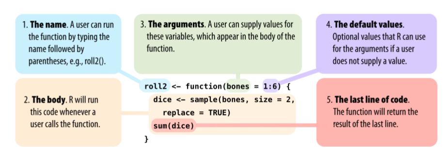
* Modified from Grolemund 2014  

R comes with many functions that you can use to do sophisticated tasks:

# built in functions
bi <- builtins()

length(bi)

## [1] 1370

sample(bi, 10)

##  [1] "unlist"            "mat.or.vec"        "close"            
##  [4] "interaction"       ".S3_methods_table" "vapply"           
##  [7] "dimnames"          "digamma"           "source"           
## [10] ".BaseNamespaceEnv"

 

Operators are functions:

1 + 1

## [1] 2

'+'(1, 1)

## [1] 2

2 * 3

## [1] 6

'*'(2, 3)

## [1] 6

 

Most commonly used R operators

Arithmetic operators:

Operator	Description
+	addition
-	subtraction
*	multiplication
/	division
^ or **	exponent
x %% y	modulus (x mod y)
x %/% y	integer division

 

1 - 2

## [1] -1

1 + 2

## [1] 3

2 ^ 2

## [1] 4

2 ** 2

## [1] 4

5 %% 2

## [1] 1

5 %/% 2

## [1] 2

 

Logical operators:

Operator	Description
<	less than
<=	less than or equal to
>	greater than
>=	greater than or equal to
==	exactly equal to
!=	not equal to
!x	Not x
x | y	x OR y
x & y	x AND y
x %in% y	match

 

1 < 2 

## [1] TRUE

1 > 2 

## [1] FALSE

1 <= 2 

## [1] TRUE

1 == 2

## [1] FALSE

1 != 2

## [1] TRUE

1 > 2 

## [1] FALSE

5 %in% 1:6

## [1] TRUE

5 %in% 1:4

## [1] FALSE

 

Most functions are vectorized:

1:6 * 1:6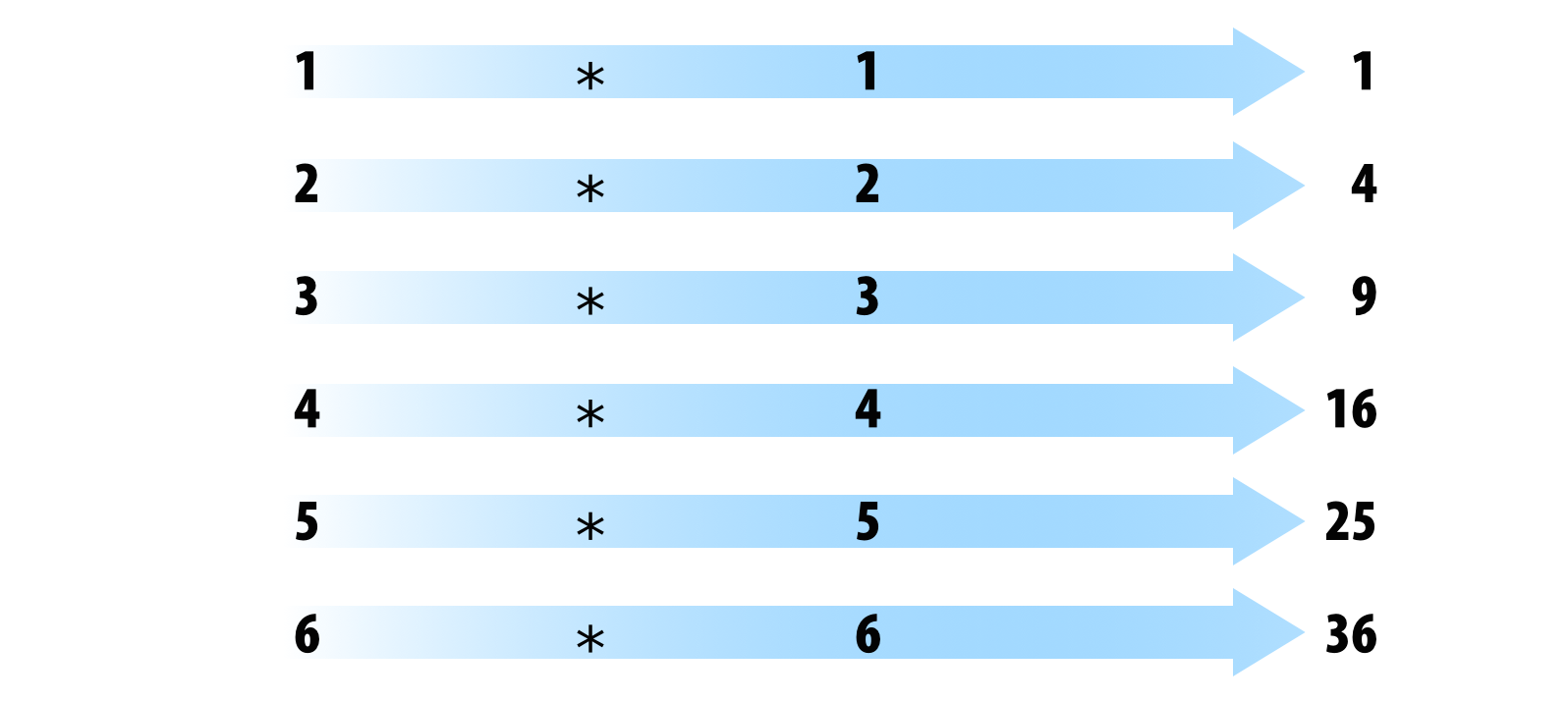

* Modified from Grolemund & Wickham 2017

 

## [1]  1  4  9 16 25 36

1:6 - 1:6

## [1] 0 0 0 0 0 0

R recycles vectors of unequal length:

1:6 * 1:5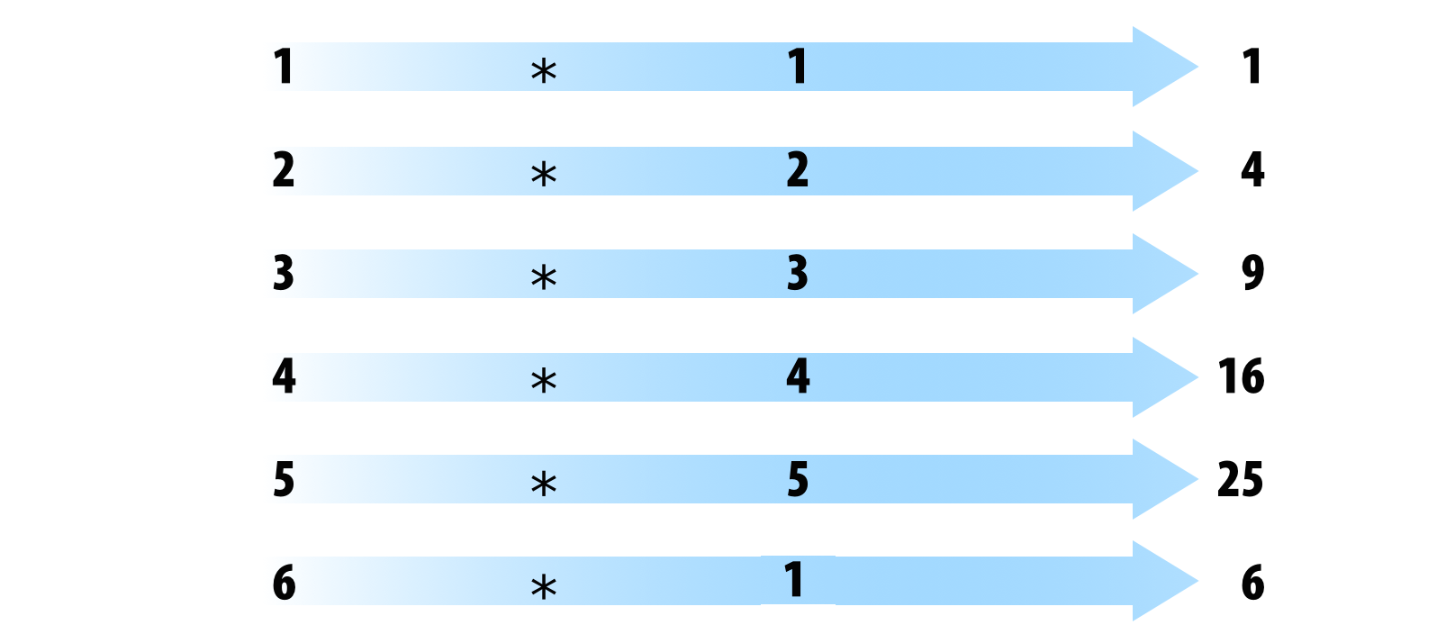

* Modified from Grolemund & Wickham 2017

 

## Warning in 1:6 * 1:5: longitud de objeto mayor no es múltiplo de la longitud de
## uno menor

## [1]  1  4  9 16 25  6

1:6 + 1:5

## Warning in 1:6 + 1:5: longitud de objeto mayor no es múltiplo de la longitud de
## uno menor

## [1]  2  4  6  8 10  7

 

---

Style matters

Based on google’s R Style Guide

File names

File names should end in .R and, of course, be meaningful:

• GOOD: predict_ad_revenue.R
• BAD: foo.R

Object names

Variables and functions:

• Lowercase
• Use an underscore (_) (HW style)
• Generally, nouns for variables and verbs for functions
• Strive for names that are concise and meaningful (not always easy)
• Avoid using names of existing functions of variables

  - GOOD: day_one: day_1, mean.day(),
  
  - BAD: dayOne, day1, firstDay_of.month, mean <- function(x) sum(x), c <- 10

 

Syntax

Spacing:

• Use spaces around operators and for argument within a function
• Always put a space after a comma, and never before (just like in regular English)
• Place a space before left parenthesis, except in a function call

  - GOOD: 
          a <- rnorm(n = 10, sd = 10, mean = 1)
          tab.prior <- table(df[df$days.from.opt < 0, "campaign.id"])
          total <- sum(x[, 1])
          total <- sum(x[1, ])
          if (debug)
          mean(1:10)
          
  - BAD: 
         a<-rnorm(n=10,sd=10,mean=1)
         tab.prior <- table(df[df$days.from.opt<0, "campaign.id"])  # Needs spaces around '<'
         tab.prior <- table(df[df$days.from.opt < 0,"campaign.id"])  # Needs a space after the comma
         tab.prior<- table(df[df$days.from.opt < 0, "campaign.id"])  # Needs a space before <-
         tab.prior<-table(df[df$days.from.opt < 0, "campaign.id"])  # Needs spaces around <-
         total <- sum(x[,1])  # Needs a space after the comma
         total <- sum(x[ ,1])  # Needs a space after the comma, not before  
         if(debug) # Needs a space before parenthesis
         mean (1:10) # ) # Extra space before parenthesis

 

Curly braces:

• An opening curly brace should never go on its own line
• Closing curly brace should always go on its own line
• You may omit curly braces when a block consists of a single statement

  - GOOD:
              if (is.null(ylim)) {
              ylim <- c(0, 0.06)
            }
                      
            if (is.null(ylim))
              ylim <- c(0, 0.06)
          
  - BAD:
            
         if (is.null(ylim)) ylim <- c(0, 0.06)
                    
         if (is.null(ylim)) {ylim <- c(0, 0.06)} 

         if (is.null(ylim)) {
           ylim <- c(0, 0.06)
           } 

 

Assigments:

• Use <-, not =

  - GOOD:
         x <- 5 
          
  - BAD:
         x = 5

 

Commenting guidelines:

• Comment your code
• Entire commented lines should begin with # and one space
• Short comments can be placed after code preceded by two spaces, #, and then one space

# Create histogram of frequency of campaigns by pct budget spent.
hist(df$pct.spent,
     breaks = "scott",  # method for choosing number of buckets
     main   = "Histogram: fraction budget spent by campaignid",
     xlab   = "Fraction of budget spent",
     ylab   = "Frequency (count of campaignids)")

 

General Layout and Ordering (google style):

• Copyright statement comment (?)
• Author comment
• File description comment, including purpose of program, inputs, and outputs
• source() and library() statements
• Function definitions
• Executed statements, if applicable (e.g., print, plot)

---

 

R documentation

Most R resources are extremely well documented. So the first source for help you should go to when writting R code is the R documention itself. All packages are documented in the same standard way. Getting familiar with the format can simplify things a lot.

Package documentation

 

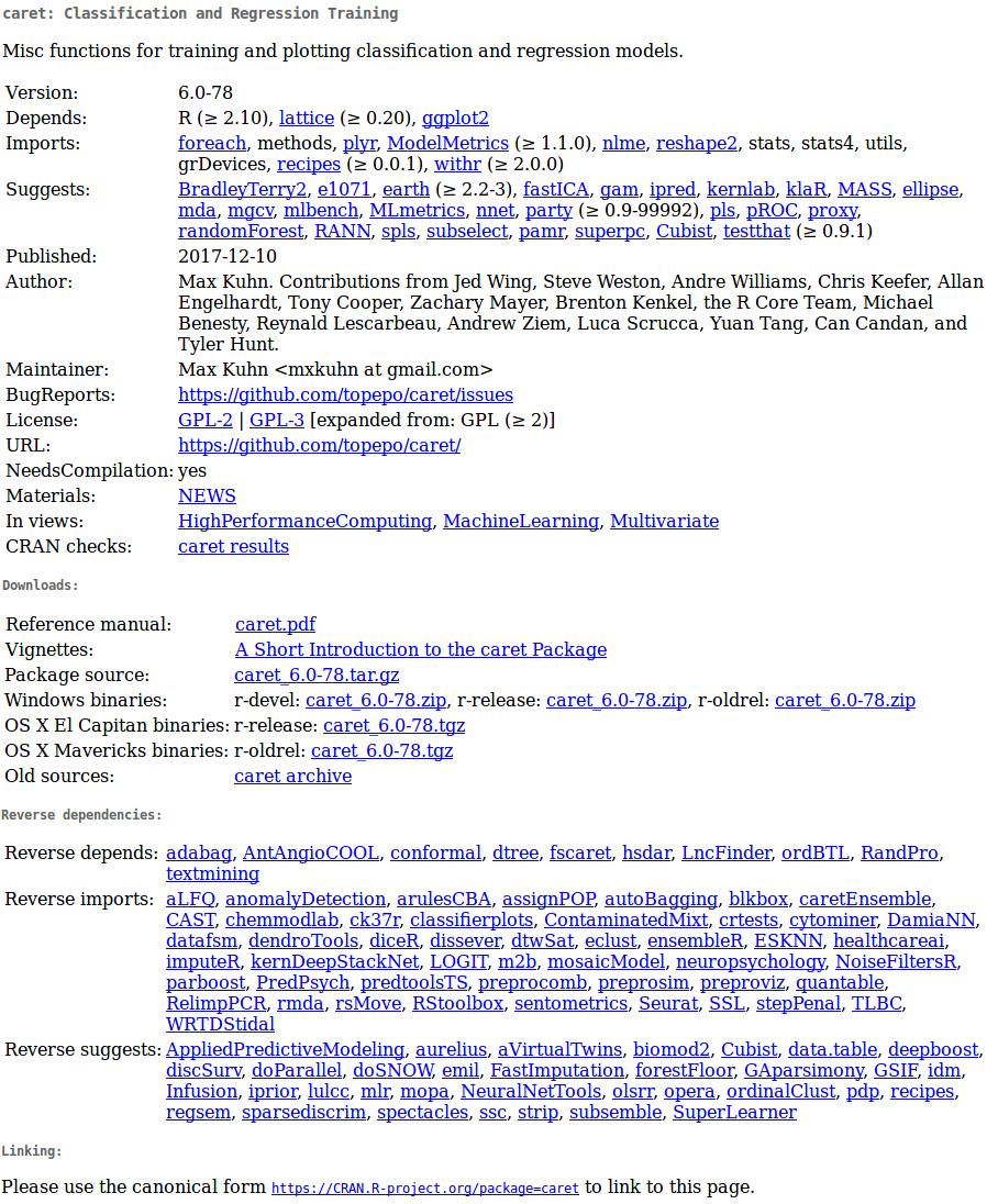
Reference manuals

Reference manuals are collections of the documentation for all functions in a package (only 1 per package):

• dynaSpec manual

• baRulho manual

 

Function documentation

All functions (default or from loaded packages) must have a documentation that follows a standard format:

?mean

help("mean")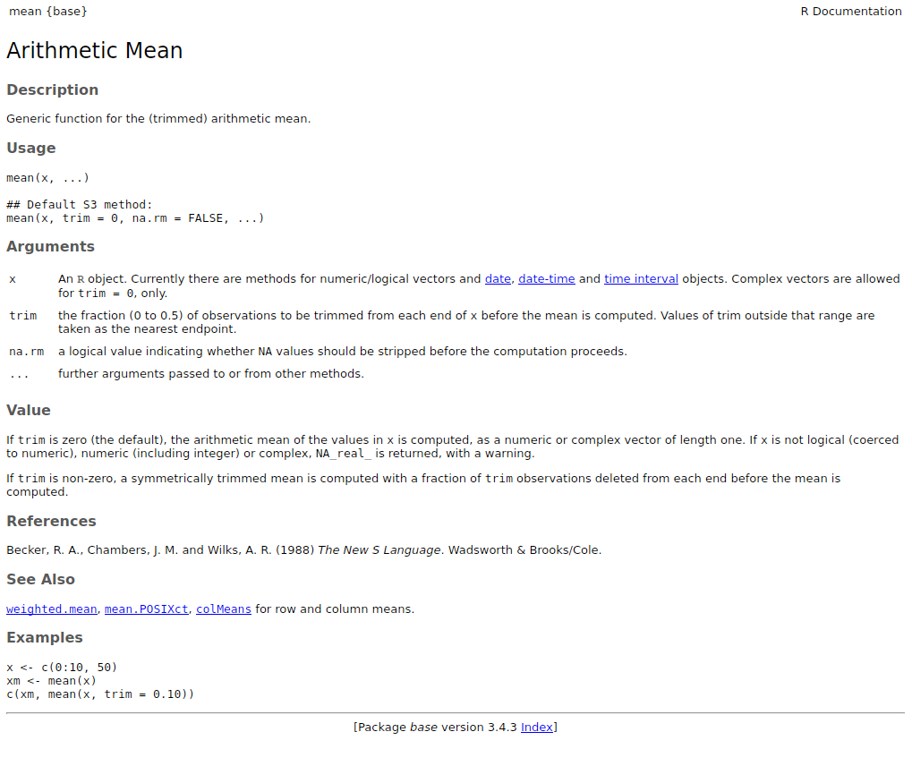

 

This documentation can also be shown in Rstudio by pressing F1 when the cursor is on the function name

 

If you don’t recall the function name try apropos():

apropos("mean")

##  [1] ".colMeans"     ".rowMeans"     "colMeans"      "kmeans"       
##  [5] "mean"          "mean.Date"     "mean.default"  "mean.difftime"
##  [9] "mean.POSIXct"  "mean.POSIXlt"  "rowMeans"      "weighted.mean"

 

Vignettes

Vignettes are illustrative documents or study cases detailing the use of a package (optional, can be several per package).

Vignettes can be called directly from R:

vgn <- browseVignettes() 

vignette()

They should also be listed in the package CRAN page.

 

Demonstrations

Packages may also include extended code demonstrations (‘demos’). To list demos in a package run demo("package name"):

demo(package="stats")

# call demo directly
demo("nlm")

 

Exercise

 

• What does the function cut() do?

• What is the breaks argument in cut() used for?

• Run the first 4 lines of code in the examples supplied in the cut() documentation

• How many vignettes does the package warbleR has?

 

---

References

• Advanced R, H Wickham
• Google’s R Style Guide
  
• Hands-On Programming with R (Grolemund, 2014)

---

 

Session information

## R version 4.1.1 (2021-08-10)
## Platform: x86_64-pc-linux-gnu (64-bit)
## Running under: Ubuntu 20.04.2 LTS
## 
## Matrix products: default
## BLAS:   /usr/lib/x86_64-linux-gnu/blas/libblas.so.3.9.0
## LAPACK: /usr/lib/x86_64-linux-gnu/lapack/liblapack.so.3.9.0
## 
## locale:
##  [1] LC_CTYPE=es_ES.UTF-8       LC_NUMERIC=C              
##  [3] LC_TIME=es_CR.UTF-8        LC_COLLATE=es_ES.UTF-8    
##  [5] LC_MONETARY=es_CR.UTF-8    LC_MESSAGES=es_ES.UTF-8   
##  [7] LC_PAPER=es_CR.UTF-8       LC_NAME=C                 
##  [9] LC_ADDRESS=C               LC_TELEPHONE=C            
## [11] LC_MEASUREMENT=es_CR.UTF-8 LC_IDENTIFICATION=C       
## 
## attached base packages:
## [1] stats     graphics  grDevices utils     datasets  methods   base     
## 
## other attached packages:
## [1] kableExtra_1.3.4 knitr_1.37      
## 
## loaded via a namespace (and not attached):
##  [1] rstudioapi_0.13   xml2_1.3.2        magrittr_2.0.2    rvest_1.0.1      
##  [5] munsell_0.5.0     viridisLite_0.4.0 colorspace_2.0-3  R6_2.5.1         
##  [9] rlang_1.0.2       fastmap_1.1.0     stringr_1.4.0     httr_1.4.2       
## [13] tools_4.1.1       webshot_0.5.2     xfun_0.30         cli_3.2.0        
## [17] jquerylib_0.1.4   systemfonts_1.0.2 htmltools_0.5.2   yaml_2.3.5       
## [21] digest_0.6.29     lifecycle_1.0.1   sass_0.4.0        glue_1.6.2       
## [25] evaluate_0.15     rmarkdown_2.10    stringi_1.7.6     compiler_4.1.1   
## [29] bslib_0.2.5.1     scales_1.1.1      svglite_2.0.0     jsonlite_1.7.2