Measures of acoustic structure

Objectives

• Learn the different methods available to quantify acoustic structure

• Understand their pros and cons

• Learn how to apply them in R

 

Acoustic signals are multidimensional traits; they vary complexly in time, frequency, amplitude and combinations of these dimensions. Generally, in biology we want to measure aspects of acoustic signals that vary in response to the factors predicted by our hypotheses. In some cases we even lack predictions for specific acoustic features and we need to evaluate the relative similarity between the variants of a signal in a population. These analyses require a diversity of tools for quantifying the multiple dimensions in which we can decompose the signals.

The warbleR package is designed to quantify the acoustic structure of a population of signals using 4 main methods of analysis. 2 of them are absolute measures of the structure:

• Spectrographic features
• Statistical descriptors of cepstral coefficients

The other 2 provide a relative similarity value between signals:

• Spectrographic cross-correlation
• Dynamic time warping

Example data

We will use the example data lbh_selec_table that comes with the package. This data frame contains the selection table of 11 long-billed hermit (Phaethornis longirostris) songs. The selection table is a data frame with the following columns:

library(warbleR)
library(viridis)
library(ggplot2)
library(ggalign)
library(PhenotypeSpace)

warbleR_options(
  wav.path = "./examples/",
  flim = c(1, 10),
  wl = 200,
  ovlp = 90,
  pb = FALSE
)

data(lbh_selec_table)

lbh_selec_table

sound.files	channel	selec	start	end	bottom.freq	top.freq
Phae.long1.wav	1	1	1.1693549	1.3423884	2.220105	8.604378
Phae.long1.wav	1	2	2.1584085	2.3214565	2.169437	8.807053
Phae.long1.wav	1	3	0.3433366	0.5182553	2.218294	8.756604
Phae.long2.wav	1	1	0.1595983	0.2921692	2.316862	8.822316
Phae.long2.wav	1	2	1.4570585	1.5832087	2.284006	8.888027
Phae.long3.wav	1	1	0.6265520	0.7577715	3.006834	8.822316
Phae.long3.wav	1	2	1.9742132	2.1043921	2.776843	8.888027
Phae.long3.wav	1	3	0.1233643	0.2545812	2.316862	9.315153
Phae.long4.wav	1	1	1.5168116	1.6622365	2.513997	9.216586
Phae.long4.wav	1	2	2.9326920	3.0768784	2.579708	10.235116
Phae.long4.wav	1	3	0.1453977	0.2904966	2.579708	9.742279

This is a catalog (made with the catalog() function) with the spectrograms of all sounds referenced in the selection table (the function saves the image file(s) in the folder in which the sound files are found):

# make a color pallete for tagging spectrograms
tag_pal <- function(x)
  mako(x,
       alpha = 0.6,
       begin = 0.1,
       end = 0.9)

# plot all annotation spectrograms in a catalog
catalog(
  lbh_selec_table,
  flim = c(1.5, 10),
  wl = 200,
  ovlp = 90,
  nrow = 4,
  ncol = 3,
  width = 12,
  height = 8,
  pb = FALSE,
  same.time.scale = TRUE,
  mar = 0.02,
  pal = mako,
  collevels = seq(-120, 0, 1),
  group.tag = "sound.files",
  tag.pal = list(tag_pal),
  spec.mar = 0.6,
  box = FALSE,
  res = 200
)

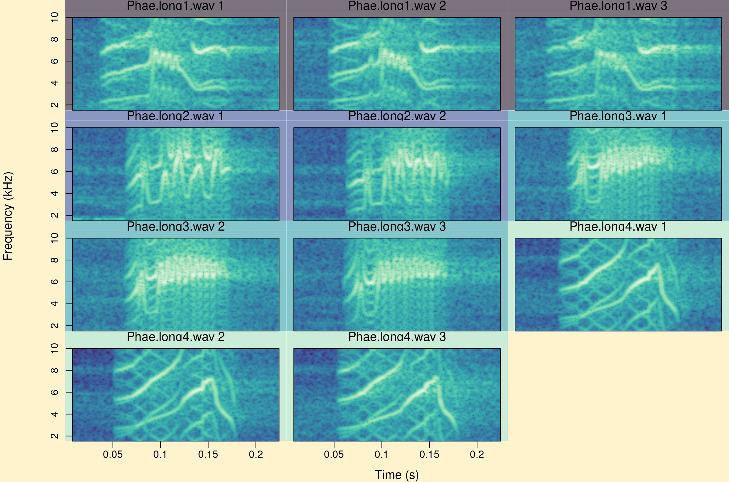
It is clear that each sound file contains a different variant of the song. We will use these data to illustrate the different methods of acoustic structure analysis available in warbleR.

1 Spectrographic features

The spectro_analysis() function measures the following spectrographic features related to amplitude distributions in time and frequency, descriptors of the fundamental and dominant frequency contours and descriptors of harmonic content:

 

1.0.1 Time and frequency (measured on the spectrogram)

• duration: signal length (in s)

• meanfreq: medium frequency. Weighted average frequency by amplitude (in kHz)

• sd: standard deviation of the amplitude weighted frequency

 

1.0.2 Energy distribution across frequencies (measured on the power spetrum)

• freq.median: medium frequency. The frequency at which the signal is divided into two frequency intervals of equal energy (in kHz)

• freq.Q25: first frequency quartile. The frequency at which the signal is divided into two frequency ranges of 25% and 75% energy respectively (in kHz)

• freq.Q75: third frequency quartile. The frequency at which the signal is divided into two frequency ranges of 75% and 25% energy respectively (in kHz)

• freq.IQR: interquartile frequency range. Frequency range between ‘freq.Q25’ and ‘freq.Q75’ (in kHz)

• sp.ent: spectral entropy. Frequency spectrum energy distribution. Pure tone ~ 0; loud ~ 1

• peakf: peak frequency. Frequency with the highest energy. This parameter can take a considerable amount of time to measure. Only generated if fast = FALSE. It provides a more accurate measurement of the peak frequency than meanpeakf(), but can be more easily affected by background noise

• meanpeakf: mean peak frequency. Frequency with the highest energy of the medium frequency spectrum (see meanspec()). Typically more consistent than peakf()

 

1.0.3 Energy distribution across time (measured on the amplitude envelope)

• time.median: average time. The time at which the signal is divided into two time intervals of equal energy (in s)

• time.Q25: first quartile. The time in which the signal is divided into two time intervals of 25% and 75% energy respectively (in s)

• time Q75: third quartile. The time in which the signal is divided into two time intervals of 75% and 25% energy respectively (in s)

• time.IQR: interquartile time range. Time range between ‘time.Q25’ and ‘time.Q75’ (in s)

• skew (skewness): Asymmetry of the amplitude distribution

• kurt (kurtosis): measure of “peakedness” of the spectrum

• time.ent: temporary entropy. Energy distribution in the time envelope. Pure tone ~ 0; loud ~ 1

• entropy: Product of the spectral and temporal entropy: sp.ent * time.ent

• sfm: spectral flatness. Similar to sp.ent (pure tone ~ 0; loud ~ 1)

• peakt: peak time. Time at which the maximum amplitude is found in the amplitude vector (in s)

1.0.4 Dominant frequency contour descriptors (measured on the spectrogram)

• meandom: average of the dominant frequency measured through the signal

• mindom: minimum dominant frequency measured through the signal

• maxdom: maximum of the dominant frequency measured through the signal

• dfrange: dominant frequency range measured through the signal

• modindx: modulation index. Calculated as the cumulative absolute difference between adjacent measurements of dominant frequencies divided by the dominant frequency range. 1 means that the signals are not modulated

• startdom: measurement of dominant frequency at the beginning of the signal

• enddom: dominant frequency measurement at the end of the signal

• dfslope: pending change in the dominant frequency over time ((enddom-startdom)/duration). The units are kHz/s

 

1.1 Optional features (if harmonicity = TRUE)

1.1.1 Fundamental frequency contour descriptors (measured on the spectrogram)

• meanfun: average of the fundamental frequency measured through the signal

• minfun: minimum fundamental frequency measured through the signal

• maxfun: maximum fundamental frequency measured through the signal

1.1.2 Harmonic content descriptors (measured on the spectrogram)

• hn_freq: average frequency of the upper ‘n’ harmonics (kHz) The number of harmonics is defined with the argument ‘nharmonics’

• hn_width: average bandwidth of the upper ‘n’ harmonics (kHz) (see analysis). The number of harmonics is defined with the argument ‘nharmonics’

• harmonics: the amount of energy in higher harmonics. The number of harmonics is defined with the argument ‘nharmonics’

• HNR: relationship between harmonics and noise (dB). A measure of harmonic content

 

We can easily measure them as follows:

# load examples
data("lbh_selec_table")

sp <- spectro_analysis(lbh_selec_table)

sp

sound.files	selec	duration	meanfreq	sd	freq.median	freq.Q25	freq.Q75	freq.IQR	time.median	time.Q25	time.Q75	time.IQR	peakt	skew	kurt	sp.ent	time.ent	entropy	sfm	meandom	mindom	maxdom	dfrange	modindx	startdom	enddom	dfslope	meanpeakf
Phae.long1.wav	1	0.1730334	5.979896	1.399059	6.327995	5.293800	6.865314	1.571513	0.0761870	0.0479696	0.1175725	0.0696029	0.0601971	1.999405	7.027830	0.9434264	0.8885049	0.8382390	0.6510692	6.481045	2.86875	8.38125	5.5125	5.979592	7.03125	2.86875	-24.056042	7.14375
Phae.long1.wav	2	0.1630480	5.997299	1.422930	6.212125	5.328746	6.880795	1.552049	0.0763491	0.0452439	0.1149950	0.0697511	0.0640956	1.918356	7.334323	0.9468217	0.8908364	0.8434632	0.6678647	6.712500	3.88125	8.49375	4.6125	4.756098	6.91875	7.25625	2.069942	6.91875
Phae.long1.wav	3	0.1749187	6.018300	1.514853	6.424759	5.150246	6.979144	1.828898	0.0893477	0.0545491	0.1279082	0.0733591	0.1232057	2.496740	11.147728	0.9450838	0.8882080	0.8394311	0.6716602	6.560194	2.30625	8.71875	6.4125	6.842105	2.30625	7.25625	28.298854	7.14375
Phae.long2.wav	1	0.1325709	6.398304	1.340412	6.595971	5.607323	7.380852	1.773529	0.0763038	0.0534126	0.1039639	0.0505512	0.0677196	1.568523	6.016392	0.9424661	0.9000328	0.8482504	0.6086184	6.510728	4.89375	7.93125	3.0375	9.703704	7.14375	6.24375	-6.788820	7.36875
Phae.long2.wav	2	0.1261502	6.308252	1.369242	6.596836	5.605837	7.207292	1.601455	0.0770280	0.0539196	0.0991735	0.0452539	0.0654738	2.470897	10.896039	0.9357725	0.9029598	0.8449650	0.6152336	6.223139	3.09375	7.70625	4.6125	7.048781	5.68125	6.46875	6.242559	6.69375
Phae.long3.wav	1	0.1312195	6.608301	1.092168	6.665328	6.063201	7.343674	1.280473	0.0641852	0.0431095	0.0890929	0.0459835	0.0526894	1.775295	6.632376	0.9301880	0.9007131	0.8378325	0.5700750	6.708750	4.89375	8.04375	3.1500	7.928571	5.68125	7.93125	17.146838	6.69375
Phae.long3.wav	2	0.1301789	6.639859	1.117356	6.674164	6.105325	7.427493	1.322168	0.0689176	0.0449879	0.0938046	0.0488167	0.0478595	1.545851	4.969900	0.9232849	0.9014187	0.8322663	0.5317422	6.532190	4.66875	8.15625	3.4875	7.870968	5.68125	6.58125	6.913561	6.69375
Phae.long3.wav	3	0.1312170	6.580739	1.253000	6.646959	6.029463	7.394054	1.364591	0.0641635	0.0402219	0.0928934	0.0526715	0.0478832	1.802520	5.886959	0.9191879	0.9013920	0.8285486	0.5258369	6.379076	2.98125	8.04375	5.0625	5.244444	2.98125	6.80625	29.150196	6.69375
Phae.long4.wav	1	0.1454249	6.219479	1.478869	6.233074	5.456261	7.305488	1.849227	0.0826911	0.0446722	0.1121557	0.0674835	0.1112052	1.274811	4.458109	0.9643357	0.8959714	0.8640172	0.7599268	6.209416	3.43125	8.71875	5.2875	7.702128	7.93125	3.43125	-30.943804	6.24375
Phae.long4.wav	2	0.1441864	6.462809	1.592876	6.338070	5.630777	7.572366	1.941589	0.0834713	0.0426842	0.1081333	0.0654491	0.1062363	1.695847	6.442755	0.9585943	0.8964128	0.8592962	0.7199148	6.386397	3.31875	9.05625	5.7375	3.921569	8.04375	3.31875	-32.770070	6.24375
Phae.long4.wav	3	0.1450989	6.122156	1.541046	6.081716	5.178639	7.239860	2.061221	0.0806173	0.0436282	0.1100189	0.0663907	0.1081220	1.083042	4.194037	0.9642064	0.8962628	0.8641823	0.7332565	6.180195	3.31875	8.60625	5.2875	6.255319	7.81875	3.31875	-31.013324	6.01875

We can reduce the dimensionality using Principal component analysis (PCA):

# run principal components
pca <- prcomp(sp[, -c(1, 2)], scale = TRUE)

# extract first 2 PCs
sp_pcs <- data.frame(sp[, 1:2], pca$x[, 1:2])

sp_pcs

sound.files	selec	PC1	PC2
Phae.long1.wav	1	-2.291437	-2.0612544
Phae.long1.wav	2	-1.442566	-1.9708581
Phae.long1.wav	3	-3.273223	-5.2403711
Phae.long2.wav	1	2.056804	0.6250836
Phae.long2.wav	2	1.787225	-1.1161183
Phae.long3.wav	1	5.149163	0.5298415
Phae.long3.wav	2	4.781227	1.0721504
Phae.long3.wav	3	4.136846	-0.2481345
Phae.long4.wav	1	-3.534622	2.7908224
Phae.long4.wav	2	-3.191386	2.5359636
Phae.long4.wav	3	-4.178032	3.0828749

The acoustic space described by this data can be easily visualized with a scatterplot:

ggplot(sp_pcs,
       aes(
         x = PC1,
         y = PC2,
         color = sound.files,
         shape =  sound.files
       )) +
  geom_point(size = 5) +
  scale_color_viridis_d(option = "G",
                        end = 0.9,
                        direction = -1) +
  theme_classic() +
  labs(x = "PC1", y = "PC2") +
  theme(legend.position = "right")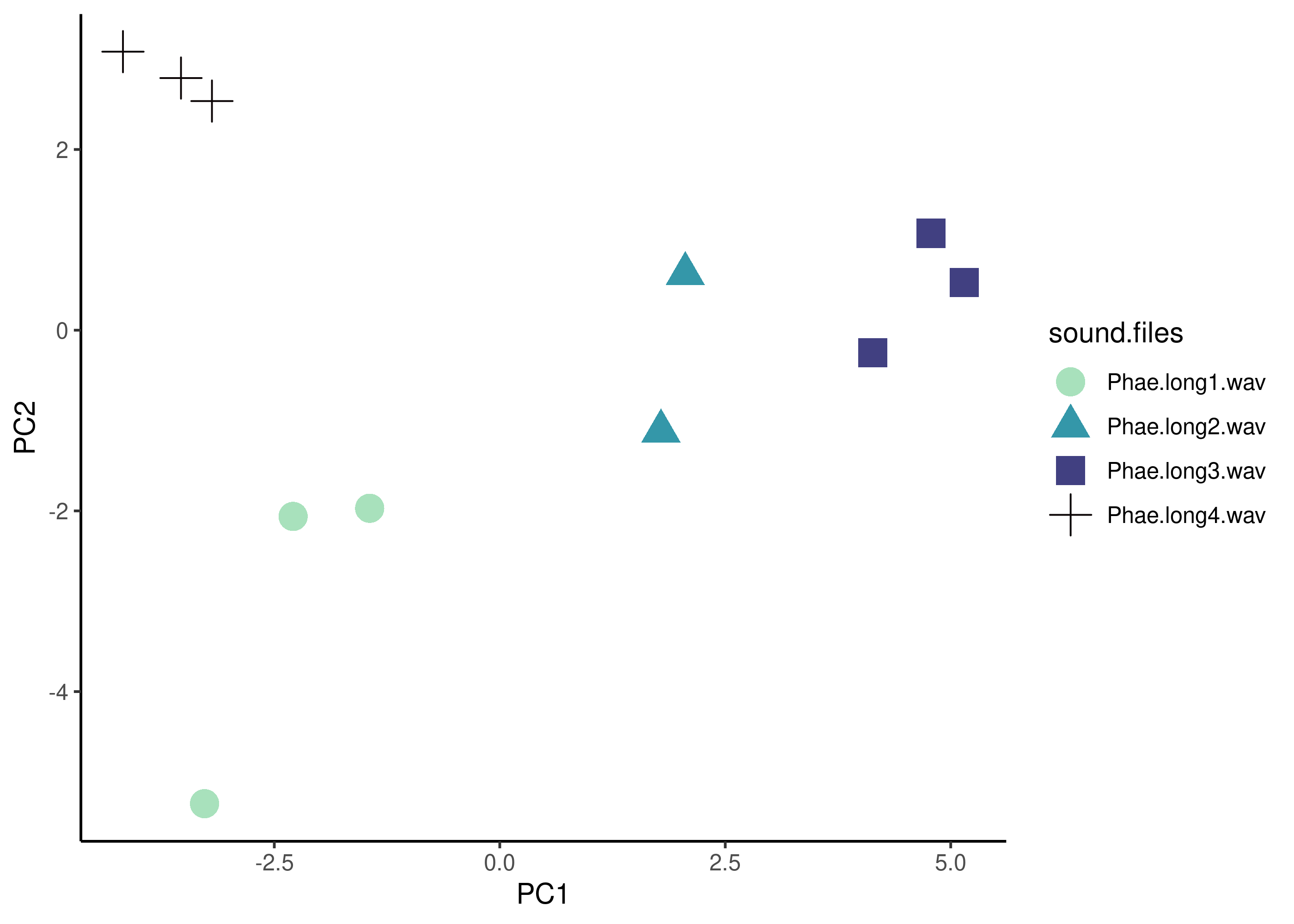

Exercise

• The features related to harmonic content were not calculated. How can we do that?

• How does measuring harmonic content affect performance?

• What does the argument ‘threshold’ do?

 

2 Statistical descriptors of cepstral coefficients

These coefficients were designed to decompose the sounds in a similar way than the human auditory system in order to facilitate speech recognition. The central idea is to compress the acoustic data maintaining only relevant information for the detection of phonetic differences. The principle refers to human hearing using the Mel logarithmic scale whose definition is based on how the human ear perceives frequency and loudness (Sueur 2018). Cepstral coefficients are literally defined as “the result of a cosine transformation of the real logarithm of short-term energy spectra expressed on a Mel frequency scale”.

The descriptive statistics that are extracted from the cepstral coefficients are: minimum, maximum, average, median, asymmetry, kurtosis and variance. It also returns the mean and variance for the first and second derivatives of the coefficients. These features are commonly used in the processing and detection of acoustic signals (e.g. Salamon et al 2014). They have been widely used for human voice analysis and its use has extended to mammalian bioacoustics, although they also appear to be useful for quantifying the structure of acoustic signals in other groups.

In warbleR we can calculate statistical descriptors of cepstral coefficients with the mfcc_stats() function:

cc <- mfcc_stats(X = lbh_selec_table)

cc

sound.files	selec	min.cc1	min.cc2	min.cc3	min.cc4	min.cc5	min.cc6	min.cc7	min.cc8	min.cc9	min.cc10	min.cc11	min.cc12	min.cc13	min.cc14	min.cc15	min.cc16	min.cc17	min.cc18	min.cc19	min.cc20	min.cc21	min.cc22	min.cc23	min.cc24	min.cc25	max.cc1	max.cc2	max.cc3	max.cc4	max.cc5	max.cc6	max.cc7	max.cc8	max.cc9	max.cc10	max.cc11	max.cc12	max.cc13	max.cc14	max.cc15	max.cc16	max.cc17	max.cc18	max.cc19	max.cc20	max.cc21	max.cc22	max.cc23	max.cc24	max.cc25	median.cc1	median.cc2	median.cc3	median.cc4	median.cc5	median.cc6	median.cc7	median.cc8	median.cc9	median.cc10	median.cc11	median.cc12	median.cc13	median.cc14	median.cc15	median.cc16	median.cc17	median.cc18	median.cc19	median.cc20	median.cc21	median.cc22	median.cc23	median.cc24	median.cc25	mean.cc1	mean.cc2	mean.cc3	mean.cc4	mean.cc5	mean.cc6	mean.cc7	mean.cc8	mean.cc9	mean.cc10	mean.cc11	mean.cc12	mean.cc13	mean.cc14	mean.cc15	mean.cc16	mean.cc17	mean.cc18	mean.cc19	mean.cc20	mean.cc21	mean.cc22	mean.cc23	mean.cc24	mean.cc25	var.cc1	var.cc2	var.cc3	var.cc4	var.cc5	var.cc6	var.cc7	var.cc8	var.cc9	var.cc10	var.cc11	var.cc12	var.cc13	var.cc14	var.cc15	var.cc16	var.cc17	var.cc18	var.cc19	var.cc20	var.cc21	var.cc22	var.cc23	var.cc24	var.cc25	skew.cc1	skew.cc2	skew.cc3	skew.cc4	skew.cc5	skew.cc6	skew.cc7	skew.cc8	skew.cc9	skew.cc10	skew.cc11	skew.cc12	skew.cc13	skew.cc14	skew.cc15	skew.cc16	skew.cc17	skew.cc18	skew.cc19	skew.cc20	skew.cc21	skew.cc22	skew.cc23	skew.cc24	skew.cc25	kurt.cc1	kurt.cc2	kurt.cc3	kurt.cc4	kurt.cc5	kurt.cc6	kurt.cc7	kurt.cc8	kurt.cc9	kurt.cc10	kurt.cc11	kurt.cc12	kurt.cc13	kurt.cc14	kurt.cc15	kurt.cc16	kurt.cc17	kurt.cc18	kurt.cc19	kurt.cc20	kurt.cc21	kurt.cc22	kurt.cc23	kurt.cc24	kurt.cc25	mean.d1.cc	var.d1.cc	mean.d2.cc	var.d2.cc
Phae.long1.wav	1	84.32923	-11.76513	-11.18492	-6.0584627	-19.48781	-18.925700	-29.78141	-20.108571	-30.013144	-35.33559	-18.78548	-14.72824	-17.34269	-15.038620	-16.88236	-19.350662	-18.31898	-22.172183	-14.48335	-18.022615	-12.746066	-11.956576	-16.452832	-11.271758	-17.689274	113.99735	-3.504852	4.9044888	14.01473	11.926071	23.15194	18.45006	18.279624	13.24953	19.780421	25.037088	11.088286	9.420685	19.068858	15.261244	27.81587	14.76590	23.18529	23.323491	13.35063	13.489834	11.386929	14.879921	17.460077	17.881148	100.78462	-8.014139	-2.523547	4.5129178	-4.654038	1.7101299	0.4097267	-8.2092001	-0.6494351	-12.2767547	3.2440322	-1.2003857	0.5455499	4.5166704	-0.3083392	-5.0343073	-0.8391115	0.1977175	5.0807704	-0.4957302	0.4521028	1.4788429	0.4990238	2.4981325	-3.1430709	101.08282	-7.858590	-2.583408	3.6987932	-4.971305	4.1609654	-2.0280573	-4.7209259	-2.8665075	-11.1703248	3.2227089	-1.6356360	-0.5039902	4.3564081	-0.1989548	-2.9284445	-1.1523253	-0.7210100	6.2913939	-0.3807152	0.3753687	1.3054995	1.0918911	2.5730086	-3.4629084	38.54742	3.080550	9.676699	24.878891	51.02731	143.44956	228.64581	92.565654	81.37786	183.97728	110.99179	31.78753	32.98640	50.46467	49.74505	101.25749	53.45791	70.55530	77.18366	58.48509	28.36997	18.42023	43.55758	36.11912	50.53745	-0.8525715	0.0070749	-0.3394632	-0.0228898	-0.0499756	0.0314614	-0.3777624	0.7563943	-0.8795527	0.1369849	0.0356844	-0.2693451	-0.5837437	-0.1670622	-0.1587374	1.0948912	-0.3489756	-0.1417061	0.0615221	-0.3280103	0.0002460	-0.3000768	-0.0950197	0.1054436	0.2366725	3.978925	2.572158	3.259741	1.969604	2.439503	1.555814	1.817494	2.429605	3.295335	1.736930	2.187305	2.322068	2.838789	2.518899	2.388298	3.845852	2.422849	3.322209	2.096780	2.617920	2.845040	2.944752	2.695023	2.404698	2.979525	-162.8716	120738.39	2274.538	13988635
Phae.long1.wav	2	86.07548	-11.91646	-12.18542	-8.6272984	-18.72726	-19.122828	-29.55422	-15.419662	-23.873777	-39.56706	-16.48812	-15.67352	-20.04686	-16.567527	-23.43945	-16.600334	-20.51312	-20.710603	-10.18992	-19.518550	-10.980131	-9.042274	-22.290707	-13.343676	-18.216693	113.72199	-4.613946	4.0046793	17.26028	11.839680	20.98899	18.18485	16.048474	13.01459	26.481963	23.840422	12.489321	12.888397	17.280133	11.552351	30.00600	26.34564	26.60756	26.783712	14.75662	12.181809	9.479065	16.702203	10.074379	27.159221	102.96939	-8.232139	-3.305544	5.3750185	-5.522622	-1.4281089	-0.8799003	-4.0623761	1.2965903	-10.9291358	0.9674887	-2.5717512	2.3195448	2.7489489	-2.4962780	-0.4686710	-1.4110075	0.3941393	4.5034699	-3.1118899	0.8915142	0.8774014	0.9537821	0.6016009	-2.3760850	102.11641	-8.110811	-3.270509	4.0824555	-5.279448	2.1963647	-3.8359976	-1.9337745	-0.1455146	-7.1102704	2.3428896	-1.8141892	0.8499174	2.1053632	-3.0172479	1.9352943	-2.4889097	0.8561653	4.7234929	-2.8633469	0.9329030	0.5541757	0.4571885	0.3962518	-1.7985663	32.69969	3.272744	12.120477	34.220961	59.92448	161.62623	190.11835	87.309406	76.27199	197.43674	100.12692	30.49991	43.78743	34.62127	64.53584	113.70042	73.03144	94.22433	84.13487	70.17767	24.55948	16.36854	71.95985	28.68820	78.75229	-0.7937595	0.0368251	-0.1836676	-0.2477335	0.2052126	0.0785791	-0.3988799	0.2427482	-0.7602454	0.2264087	0.2118971	0.0189160	-0.6390020	-0.1645549	-0.4137205	1.0354560	0.1110707	0.2029748	0.2052125	0.0468125	-0.1614243	-0.0904110	-0.6670217	-0.2735971	0.9766275	3.499764	2.309498	2.535486	2.574509	2.153644	1.473513	1.943041	1.637756	2.839401	2.478765	2.033868	3.389931	2.726985	3.201433	2.395783	3.746845	3.235674	3.263642	2.040132	2.243469	2.405112	2.403771	3.177252	2.332764	4.299571	-162.7222	125044.72	2358.420	14610321
Phae.long1.wav	3	84.71447	-12.86693	-12.37385	-6.6677525	-17.93314	-15.855967	-28.84733	-18.620027	-20.857060	-38.24592	-16.96329	-12.18738	-22.86534	-7.317589	-20.06833	-22.161444	-19.36095	-21.741610	-10.87104	-12.149563	-14.662678	-7.931532	-16.423956	-10.964721	-21.643870	108.18040	-2.964319	4.0996661	14.58979	9.184255	23.05499	20.77710	17.371439	14.50500	18.461626	22.936062	16.707360	13.913267	21.969152	15.766074	21.96113	11.44151	15.36057	24.586317	13.99253	13.378289	12.853060	17.257267	12.082475	20.207047	98.16825	-9.028246	-3.016906	3.5703002	-5.831004	1.3350682	0.7441784	-5.8756895	-1.9412309	-11.3615555	3.6082495	0.7845383	1.0138900	3.5563993	-0.9615083	-4.9571527	-0.2061702	0.3086402	3.8898702	0.2277695	-0.2069073	1.0601127	2.3452034	1.8802654	-2.8945657	97.81067	-8.405651	-2.853761	2.6311424	-4.651573	4.8392030	-2.3114324	-2.8713025	-2.5946477	-10.7281817	3.0926057	0.7038435	0.4572550	4.2125981	-0.7717674	-2.7353614	-1.0883229	-0.4691156	4.9406418	0.5472174	0.6017814	0.7476270	2.2475173	1.4723863	-3.0864121	27.66152	5.455827	13.984391	26.119854	47.45200	145.84450	173.16803	82.233643	59.94727	209.29478	78.04604	33.45872	49.39895	41.80205	58.96178	92.02909	46.43705	57.16307	57.65391	36.67725	24.79103	18.71207	41.84955	29.14779	46.46215	-0.6098012	0.4598246	-0.2788199	0.0353535	0.2516610	0.1118688	-0.3816367	0.6782386	-0.1451220	-0.1623321	-0.0378343	0.0683836	-0.7565889	0.7368333	-0.2841870	0.7107961	-0.4949666	-0.4362038	0.4053479	-0.0378969	0.1268823	0.2473709	-0.4867252	-0.1591703	0.4457043	2.959010	2.274255	2.543097	2.113162	2.188736	1.531366	1.978457	2.438865	2.724626	2.068398	1.966382	2.968897	4.250107	3.039181	2.639594	3.085653	2.924919	2.873747	2.593373	2.389900	3.110694	2.716579	3.275660	2.298071	4.609402	-156.7522	112731.22	2207.924	13414726
Phae.long2.wav	1	50.56041	-18.77867	-19.18023	-5.1156831	-15.31201	-14.853539	-19.67227	-11.337266	-14.293743	-19.31601	-18.31851	-11.52312	-11.87761	-11.474193	-15.59440	-13.046359	-13.47313	-12.666432	-17.30676	-16.478239	-10.301012	-8.518116	-12.098098	-9.938733	-21.899395	95.82797	-1.476256	0.5356803	14.14524	4.987772	18.03277	12.57080	9.708234	15.57415	14.235474	14.932578	11.346420	13.755391	10.716971	15.203273	15.99467	14.70524	19.57898	15.465918	15.76738	17.087750	9.627947	11.107409	14.562106	5.685059	89.56016	-13.281239	-6.201262	6.3350504	-6.726423	2.5687735	-0.8244336	0.2318829	-1.7580541	0.1028389	0.4976419	-0.3414484	1.4830689	-0.3087596	1.0895142	2.8904778	1.5452386	-0.6254576	-0.6399199	-0.1125934	1.0698166	-1.2195655	1.1398485	-0.5621275	-2.9780041	87.54748	-12.254268	-6.689966	4.8505420	-5.763817	2.1524591	-0.9377664	0.0118461	0.0193052	-0.5631844	-0.1486082	-0.3659984	1.0885994	-0.8844645	0.5384982	2.1560721	1.2031469	0.2965713	-1.1924972	0.4344829	1.9361923	-0.9634357	1.2080221	-0.3801088	-3.1717546	55.43443	14.197314	16.523243	31.191793	27.36259	68.21222	46.19293	20.532498	40.28372	45.91169	74.09408	26.48263	36.44235	21.84555	38.27894	28.54412	30.11865	36.06963	33.54773	29.39322	31.44592	14.06754	24.09755	25.55710	29.30412	-2.3617737	0.5620661	-0.7853844	-0.3253047	0.2921540	-0.2184238	-0.4646152	-0.4495660	0.5446993	-0.5564179	-0.2611293	0.0441089	0.0447220	-0.3642512	-0.1266515	-0.4195171	-0.1044080	0.8177531	-0.1788509	-0.1490543	0.2207317	0.2935838	-0.2534314	0.6611163	-0.7195757	10.387312	2.523812	3.744378	1.698074	1.992397	2.233481	3.220366	2.799218	2.868719	3.223175	2.366506	2.316063	2.252824	2.680087	3.092792	3.440594	2.869778	4.211831	3.825819	3.657709	2.519131	2.689710	2.733973	3.322531	3.460724	-139.5949	89559.79	1997.491	11269953
Phae.long2.wav	2	69.23577	-17.18596	-20.25226	-3.7917317	-13.67741	-17.062368	-17.69824	-9.737039	-9.347726	-17.34610	-18.18316	-13.37309	-13.09030	-14.342290	-27.31758	-7.811027	-25.92640	-12.031356	-11.93306	-14.425461	-13.885818	-10.478242	-15.213300	-12.064791	-10.104834	99.97835	-4.534624	0.6537113	14.64448	5.035473	14.83004	12.36953	7.862668	16.93760	16.292855	6.457178	7.007890	8.478286	15.513147	27.147724	28.06045	12.82798	12.55751	19.160344	16.53261	6.806786	11.746044	7.754506	7.473303	16.955569	93.62319	-12.426364	-6.821915	6.3893860	-7.186507	2.4640075	1.4933313	0.9153600	3.0598443	-3.5772945	-2.7305020	-1.6300288	-5.2094337	-0.8965981	1.6895035	2.3893437	-0.9681590	-2.3933031	2.6390477	-0.3572365	-2.6157354	0.7066969	-1.5801441	-2.8620984	-0.0191788	91.53344	-10.863905	-7.527386	5.9027922	-6.464367	1.9244645	-0.0164966	1.0469669	3.1630834	-3.8855019	-2.9781009	-2.2099903	-4.3612298	-0.5546178	2.2416490	3.4286326	-1.4016094	-1.4672608	2.5565898	0.2292764	-2.4664863	0.1968881	-1.9062477	-3.2960670	0.6406991	42.73550	15.345963	19.913883	24.344033	27.18264	60.09685	52.08649	9.928084	41.39179	62.20534	25.28970	17.17876	23.13800	38.11626	75.92628	56.07860	60.29012	24.88702	28.85301	41.57108	14.55141	24.51716	26.07821	16.32374	26.10237	-0.9733968	0.3680001	-0.8780162	-0.2218139	0.6471153	-0.4018160	-0.9860828	-0.4577860	0.0500170	0.5902452	-0.3561700	-0.3136212	0.4138770	0.1423488	0.0932327	0.9353019	-1.2559760	0.5598416	0.0464672	0.1264826	-0.2631874	-0.1127727	-0.4960467	-0.0491214	0.9040419	3.545202	1.599688	3.474896	1.883349	2.362472	2.373087	3.289100	3.615628	2.182782	3.277128	2.785593	2.535871	2.494026	2.737171	5.351909	3.692174	4.843621	2.994884	3.474904	3.118363	3.011344	2.785522	2.839144	2.718442	4.140334	-142.0430	98525.41	2216.821	11213543
Phae.long3.wav	1	51.52696	-18.48908	-13.54987	0.1644875	-16.40398	-7.595591	-14.27574	-13.213955	-5.091165	-22.49984	-12.61909	-10.28927	-13.54220	-11.767158	-16.44382	-12.936966	-12.66129	-9.618623	-32.60175	-7.317495	-9.127416	-8.994948	-13.015914	-12.708262	-20.945804	91.03291	-6.438211	4.1405479	14.33518	4.606884	13.01582	11.18171	8.266875	16.40768	8.103246	9.485075	9.574047	8.639773	10.709409	11.329384	11.18601	10.36107	10.71221	9.950225	16.03712	24.730990	11.957692	9.093840	21.792011	15.059743	83.39758	-14.844842	-1.573749	7.1924013	-11.810949	7.0300692	-2.1941132	-1.7703202	2.0828468	-2.5327296	-0.7059684	0.3015867	-0.0640079	-0.6900560	1.0762733	-1.1077216	0.4657508	-0.3412012	-1.1536515	0.1696893	0.0833877	0.3784441	0.2870068	-0.1596489	-0.2142131	80.68792	-14.271362	-2.618999	7.0638940	-9.956171	5.6958684	-1.7031731	-1.5878484	3.2049362	-2.8055485	-0.9146070	-0.2788690	-0.0414812	-0.6791649	0.6176580	-1.0845294	0.2814645	-0.1251147	-2.6923536	0.3492016	0.3582097	0.1590165	-0.1397560	0.3851191	-1.0172323	66.70615	6.369703	18.995024	10.241030	23.52605	29.71595	32.12247	13.928651	22.63694	23.42001	26.71856	18.26408	20.07234	23.35500	26.39624	19.14299	23.76156	24.56074	70.11466	22.99117	43.60260	17.67860	21.30309	37.59117	41.89435	-1.4009528	0.7010760	-0.7045305	-0.1574926	1.5154837	-0.7520569	0.4028089	-0.0182238	0.7948237	-1.3661896	-0.2498680	-0.2481627	-0.4269518	-0.2017573	-0.7938926	0.0193557	-0.4020360	0.3084959	-1.4577410	0.8179731	1.3592290	-0.0870922	-0.5356686	1.1259595	-1.1072573	4.357722	2.810805	2.649706	2.619563	4.438030	2.480966	2.730453	3.850931	3.129568	7.021544	2.527106	2.478784	3.173013	2.777882	4.113397	3.492418	2.974481	2.135857	5.292465	3.666222	5.296414	2.925071	2.714289	5.456608	4.853802	-125.8625	76790.36	1904.035	9282622
Phae.long3.wav	2	52.65548	-18.25355	-15.46921	-0.9814104	-16.17827	-11.888869	-16.43251	-12.413136	-13.303840	-18.75192	-14.12018	-9.94332	-15.28994	-12.331302	-15.61214	-18.423967	-15.98526	-5.863614	-28.96201	-15.711890	-8.452064	-15.948944	-11.434859	-9.863952	-20.625615	89.25353	-6.267069	3.5404749	15.45726	3.923592	13.21030	15.00087	5.169150	12.97379	15.827433	8.115085	9.779450	14.480119	14.525023	12.480762	15.99009	11.95247	15.40194	9.997352	13.60333	19.515747	13.013623	12.235432	24.335281	8.532834	83.94096	-14.785131	-1.626893	8.0511617	-11.939951	7.3666675	-1.5767325	-1.9304223	3.9549825	-2.3628779	-2.2937143	0.0689487	0.0419978	0.5506128	2.6936255	-0.0828549	-0.7624452	1.5933829	-1.3107263	1.6486724	-1.0636650	-0.2454464	1.3396674	-1.7917913	-0.2708519	82.21010	-13.854677	-3.431409	7.7150520	-9.685058	5.3855526	-1.2871304	-2.4902302	3.7755805	-2.3687067	-2.3079403	-0.2260396	0.2929752	0.3122023	2.0454844	-0.6811508	-0.4060026	2.1806622	-1.9948232	1.2881456	-0.3267198	-0.7317912	0.8438387	-0.8889085	-0.8361620	42.25413	8.560160	21.123699	11.025058	31.26867	30.94029	35.54967	11.817944	26.23967	25.55947	21.88716	22.68222	33.16704	24.62160	22.34397	30.74143	33.72703	22.44852	47.16585	34.92344	23.26969	23.58834	22.45083	35.62439	29.97117	-1.8930677	0.7772158	-0.8901376	-0.6048479	1.2768606	-1.2004938	0.0747053	-0.4227167	-0.6352537	-0.1500344	-0.0730368	0.0198622	0.0637853	0.0755629	-0.8779759	-0.4276955	-0.2752871	0.5433153	-1.3120250	-0.3899823	1.5951218	-0.4461833	-0.2426493	2.1671706	-1.2672366	7.269170	2.738719	2.834298	3.106652	3.141681	3.639527	3.305778	3.084076	3.757768	6.197029	2.777729	2.279314	2.980824	3.161024	4.942372	4.732342	2.939234	2.815338	6.004826	2.879276	6.931951	3.576478	2.834893	9.005364	5.273010	-128.3608	78964.35	1944.363	9439147
Phae.long3.wav	3	63.52696	-17.43387	-14.57354	0.1866403	-15.93326	-14.396968	-18.36977	-11.647362	-13.343003	-17.98165	-13.11832	-16.41835	-20.33493	-12.775589	-11.20505	-18.584587	-20.62499	-13.964906	-12.06025	-4.988363	-16.109423	-10.213555	-8.516935	-18.866201	-8.701287	91.12650	-7.503753	2.5826560	13.48428	2.834422	13.10069	13.65352	7.302118	16.15262	20.472092	9.671298	10.719213	9.769547	9.010339	9.883183	15.91783	12.01769	12.32896	18.515104	15.44906	9.016017	6.910449	11.349493	5.825247	14.245435	85.51208	-13.948072	-1.998810	7.8273577	-11.837170	7.9332887	-1.2026988	-2.1468697	3.1807107	-0.3384937	0.5821092	1.6764583	-0.3457622	-2.1694142	0.1874178	0.6440910	-0.4249719	-0.9916752	-1.5969691	2.9801660	-1.2317481	0.5436020	1.7971479	-0.7717557	-0.4096777	83.58466	-13.343884	-3.480298	7.6206982	-9.972402	4.7428909	-1.4516448	-2.0991832	3.3138790	0.5980103	-0.5171419	0.8157284	-1.0814442	-2.0648980	0.1486486	0.6509199	-0.3674902	-0.4438106	-1.2793043	2.9934971	-1.7243883	-0.2204965	1.5920567	-1.8211853	-0.1166597	38.26609	6.180594	19.588460	6.252635	23.15894	46.70831	34.22287	12.178370	23.56747	38.06949	26.36688	25.49769	36.48648	20.44102	17.02402	31.61947	36.24182	29.78152	39.96716	23.83514	23.49238	16.21960	17.51334	21.88707	17.32209	-1.3816749	0.5840598	-0.8610223	-0.3178518	1.4011049	-1.1539001	-0.1064684	-0.0661053	-0.4368150	0.6554118	-0.4674317	-1.2386606	-0.7150418	0.0684964	-0.1159066	-0.2000664	-0.5671129	0.1496434	0.9414522	0.4587045	-0.7037730	-0.4643647	-0.1825552	-1.5298169	0.5314529	4.343781	2.312242	2.915892	3.155969	3.884295	3.095343	3.790482	3.333604	4.731681	6.012400	2.580577	4.922548	3.601541	2.964935	3.123543	4.569744	3.543262	2.893773	3.845489	2.555675	3.552395	2.311025	2.649072	6.034749	3.781649	-129.6083	82306.84	2000.256	9816630
Phae.long4.wav	1	81.17215	-13.36883	-14.32334	-11.2320300	-21.52305	-26.124102	-18.05137	-22.670714	-35.172175	-21.21141	-28.89065	-13.84315	-14.23210	-20.236207	-28.90261	-33.119291	-31.18754	-22.665818	-21.62963	-14.673295	-9.679038	-12.263665	-14.691732	-13.439850	-15.336906	108.29921	-2.380876	5.1480565	16.00147	17.696067	25.97502	28.93749	16.489024	20.13634	38.976446	24.093448	13.231904	22.257771	18.321101	23.887375	26.77188	23.13669	21.54162	18.211784	21.22086	19.988181	12.688617	14.944629	14.155653	12.275442	97.53010	-8.899641	-4.317321	1.2989451	-6.241419	-0.8226447	-0.6885103	1.4713862	1.4524089	-0.3251444	3.6198024	-0.8311248	0.3989674	0.9558217	0.6628059	0.2776693	-1.7683483	-2.0984331	1.1769481	-0.2437460	-0.1247434	1.8517956	1.4611222	1.4174313	-2.0160800	97.51269	-8.327846	-4.516365	1.8982430	-4.664118	0.5742034	0.8859148	-1.1323628	-3.7109920	1.8688164	1.7046859	-0.6551707	1.0868581	1.0509441	0.4126990	-1.5140302	-2.0060895	-1.8214670	0.1645343	0.6260965	1.1556291	2.1507938	0.7881952	1.1083693	-2.4252677	20.76587	6.457194	20.796837	37.013566	104.13563	210.47161	130.82306	91.173299	235.12157	214.58224	145.76044	45.72456	66.99274	69.16793	164.63625	220.09873	117.15945	73.78062	73.86750	62.68677	33.68980	20.75617	39.16623	34.48815	34.11364	-0.4807034	0.5421475	0.0438345	0.1902813	0.2445038	-0.1111487	0.4616688	-0.4352715	-0.6308532	0.5428213	-0.3824620	0.2214837	0.1234758	-0.1601147	-0.3068665	-0.3711681	0.1123062	0.0542471	-0.4097968	0.6422774	1.0350717	-0.0875763	-0.0956040	-0.0911201	-0.0404165	4.419232	2.571636	2.702961	2.563584	1.968245	1.689001	2.557529	2.212657	2.168318	2.549528	2.553938	2.109329	2.098725	2.811059	2.180414	2.540761	3.042899	2.909990	2.772233	2.916813	3.810587	3.135353	2.707688	2.576292	2.502401	-154.9780	113957.89	2232.101	14009335
Phae.long4.wav	2	85.93936	-14.02047	-15.27076	-10.5223514	-21.86064	-26.243661	-16.96860	-20.261418	-36.413874	-23.77254	-31.68066	-11.46582	-21.10015	-22.447486	-29.29393	-35.520761	-23.81466	-22.990313	-18.68782	-15.799625	-13.474434	-10.433447	-14.891138	-14.433316	-15.925166	110.11022	-2.888071	6.3154347	15.49963	17.182754	23.51133	26.58182	13.639927	19.19507	37.673677	24.696463	13.765457	18.146237	21.112545	28.348188	27.94444	24.87239	22.86546	20.101624	19.59156	18.809891	11.751474	13.824306	14.065797	14.749977	97.62676	-9.075638	-4.180906	0.8455709	-5.464755	-3.8783404	0.2011186	2.4132025	0.8420818	3.8453213	3.6287976	-0.3849610	0.3042227	0.3793168	0.9711272	0.1646577	-1.6891571	-1.4415768	2.3309450	-0.3271556	-0.6194160	1.1803271	-0.4432385	2.5612843	-2.3673988	97.69409	-8.629931	-4.223445	0.9874605	-4.946718	0.4212339	0.9734149	-0.9115828	-3.0815390	3.9563844	0.6744244	-0.2094277	0.9697767	1.2571860	0.3891992	-0.8064589	-0.9359416	-1.3903643	1.7194488	0.9394113	0.9244046	1.5109870	-0.1368488	2.2985079	-2.0471891	17.53077	5.755176	23.388071	35.774561	106.22716	213.03310	109.73196	88.997339	230.46437	213.92753	184.07761	36.39303	63.59556	93.95415	172.02878	220.11469	103.62913	80.62873	64.42422	61.13239	49.90626	20.17111	29.70700	40.19999	30.50474	0.2243093	0.4586838	0.0530041	0.0998925	0.1729316	0.0212245	0.2581881	-0.4631797	-0.7580968	0.2449392	-0.2923182	0.1278012	-0.1615675	0.0110015	-0.2495133	-0.4236119	0.4903018	0.0939729	-0.0785067	0.4191953	0.6288227	0.0016867	0.0707094	-0.3447260	0.3036929	3.950107	2.781237	2.675812	2.269614	1.914863	1.628221	2.401728	1.906990	2.459879	2.356779	2.187576	2.259377	2.426807	2.712683	2.404569	2.661049	3.155811	2.682496	2.704227	2.672580	2.741615	2.677712	3.087750	2.703029	2.962267	-154.4238	114845.97	2256.109	14157377
Phae.long4.wav	3	79.26665	-12.80419	-17.38993	-9.1865953	-22.10634	-23.168022	-21.52971	-17.775317	-33.515447	-16.75138	-21.45461	-17.72236	-18.61181	-25.293114	-24.76783	-32.651173	-17.66339	-20.192774	-17.69250	-12.900804	-13.454919	-8.309600	-18.038889	-12.132479	-18.855531	103.38287	-2.418141	4.9158186	16.55906	16.961050	24.28676	27.11997	13.883459	15.48901	36.938046	22.377769	13.133743	15.103839	24.859209	27.855612	24.87172	19.61238	16.24134	25.142440	20.91978	15.526477	11.448421	16.093285	11.618132	15.042704	93.31006	-8.253301	-5.133685	2.6243344	-5.454540	-1.8141510	-0.1533529	-0.6834088	-1.9405703	-0.0492234	6.0518700	1.1188716	1.2974693	1.0912988	-0.0965371	-1.2181218	-1.0935165	-1.8645593	2.1029980	1.5365135	-2.5229097	0.4406871	0.9182953	0.2588781	-1.8460634	93.50548	-7.961212	-4.915597	2.6947909	-4.828739	-0.2335291	0.2235244	-1.6375964	-5.8615842	3.2727209	3.5683672	0.0112065	1.2587745	0.4999968	-0.3752456	-1.8739761	-0.2379464	-1.9890846	1.4523510	2.1725026	-1.0218243	0.7895443	0.8952665	0.0606613	-1.6922789	17.57932	5.824846	21.306269	35.872770	100.32666	198.66160	150.15671	82.012748	176.94881	183.95851	141.62882	42.73552	53.34466	80.98733	131.01281	185.14814	73.94438	66.10613	74.20800	57.13816	38.63585	19.43314	41.18653	29.34954	34.09512	-0.1872895	0.4808115	-0.1492917	0.2137390	0.1219909	0.0595207	0.2072385	-0.1410997	-0.6087014	0.5782024	-0.4875747	-0.3851620	-0.5099451	-0.4866950	-0.0790980	-0.3480380	0.2234092	-0.1314042	0.1389349	0.2740072	0.4294181	0.2147506	-0.6054106	0.0163128	-0.2643390	3.599611	2.380272	3.195556	2.393710	1.969326	1.714357	2.303348	1.774513	2.195820	2.359424	2.138020	2.494256	3.193837	4.141875	2.705730	2.595008	2.324069	2.590252	3.128677	2.322027	2.671382	2.453939	4.095454	2.486660	3.300506	-148.1063	106126.37	2177.672	12979235

Similarly to the spectrographic features, we can reduce the dimensionality of the cepstral coefficients using PCA:

# run principal components
pca <- prcomp(cc[, -c(1, 2)], scale = TRUE)

# extract first 2 PCs
cc_pcs <- data.frame(cc[, 1:2], pca$x[, 1:2])

cc_pcs

sound.files	selec	PC1	PC2
Phae.long1.wav	1	-6.701782	7.1012038
Phae.long1.wav	2	-7.749850	7.2089600
Phae.long1.wav	3	-5.494403	6.7191726
Phae.long2.wav	1	5.841362	-1.1111075
Phae.long2.wav	2	6.214191	-3.2835692
Phae.long3.wav	1	11.019149	0.7766946
Phae.long3.wav	2	11.812781	0.0107302
Phae.long3.wav	3	9.545288	0.8442370
Phae.long4.wav	1	-8.182452	-6.9390541
Phae.long4.wav	2	-8.797570	-6.7546117
Phae.long4.wav	3	-7.506716	-4.5726558

Again, this simplified acoustic space can be easily visualized with a scatterplot:

ggplot(cc_pcs,
       aes(
         x = PC1,
         y = PC2,
         color = sound.files,
         shape =  sound.files
       )) +
  geom_point(size = 5) +
  scale_color_viridis_d(option = "G",
                        end = 0.9,
                        direction = -1) +
  theme_classic() +
  labs(x = "PC1", y = "PC2") +
  theme(legend.position = "right")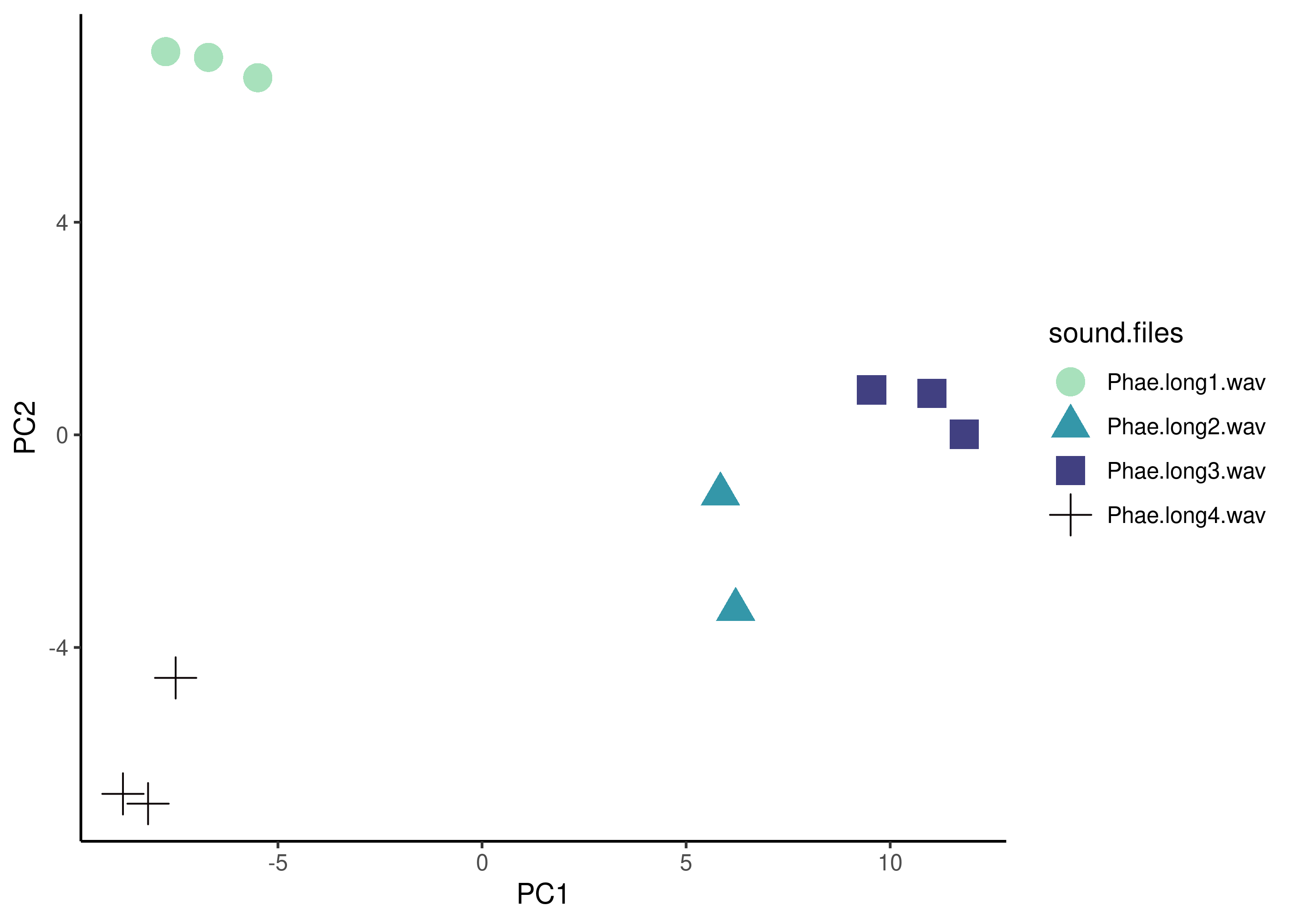

3 (Spectrographic) cross correlation

This analysis correlates the amplitude values in the frequency and time space pairwise for all signals in a selection table. The correlation represents a measure of spectrographic similarity of the signals:

xcor <- cross_correlation(X = lbh_selec_table)

xcor

	Phae.long1.wav-1	Phae.long1.wav-2	Phae.long1.wav-3	Phae.long2.wav-1	Phae.long2.wav-2	Phae.long3.wav-1	Phae.long3.wav-2	Phae.long3.wav-3	Phae.long4.wav-1	Phae.long4.wav-2	Phae.long4.wav-3
Phae.long1.wav-1	1.0000000	0.6638508	0.6491063	0.1946160	0.2615196	0.3339740	0.2992381	0.3383126	0.1834400	0.1577694	0.2048526
Phae.long1.wav-2	0.6638508	1.0000000	0.7118060	0.2458648	0.2660671	0.3280084	0.2835975	0.3409463	0.0954318	0.0913951	0.1307878
Phae.long1.wav-3	0.6491063	0.7118060	1.0000000	0.2442306	0.3080008	0.3520654	0.3175826	0.3426542	0.1610333	0.1476679	0.1905664
Phae.long2.wav-1	0.1946160	0.2458648	0.2442306	1.0000000	0.5949237	0.5617453	0.5729078	0.5002876	0.2741691	0.2470523	0.2871090
Phae.long2.wav-2	0.2615196	0.2660671	0.3080008	0.5949237	1.0000000	0.5098819	0.5427296	0.5103951	0.2097443	0.1923960	0.2334284
Phae.long3.wav-1	0.3339740	0.3280084	0.3520654	0.5617453	0.5098819	1.0000000	0.7865409	0.7247518	0.1340282	0.1314775	0.1516756
Phae.long3.wav-2	0.2992381	0.2835975	0.3175826	0.5729078	0.5427296	0.7865409	1.0000000	0.7259070	0.1766590	0.1735262	0.1979071
Phae.long3.wav-3	0.3383126	0.3409463	0.3426542	0.5002876	0.5103951	0.7247518	0.7259070	1.0000000	0.1879558	0.1754047	0.2092285
Phae.long4.wav-1	0.1834400	0.0954318	0.1610333	0.2741691	0.2097443	0.1340282	0.1766590	0.1879558	1.0000000	0.5277140	0.8161098
Phae.long4.wav-2	0.1577694	0.0913951	0.1476679	0.2470523	0.1923960	0.1314775	0.1735262	0.1754047	0.5277140	1.0000000	0.5197698
Phae.long4.wav-3	0.2048526	0.1307878	0.1905664	0.2871090	0.2334284	0.1516756	0.1979071	0.2092285	0.8161098	0.5197698	1.0000000

The similarity matrix returned by the function can be visualized as a heatmap:

# present xcor as a heatmap using ggplot2
ggheatmap(xcor) +
  scale_fill_viridis_c(
    option = "G",
    direction = 1,
    begin = 0.1,
    end = 0.8
  ) +
  theme(axis.text.x = element_text(angle = 90))

→ heatmap built with `geom_tile()`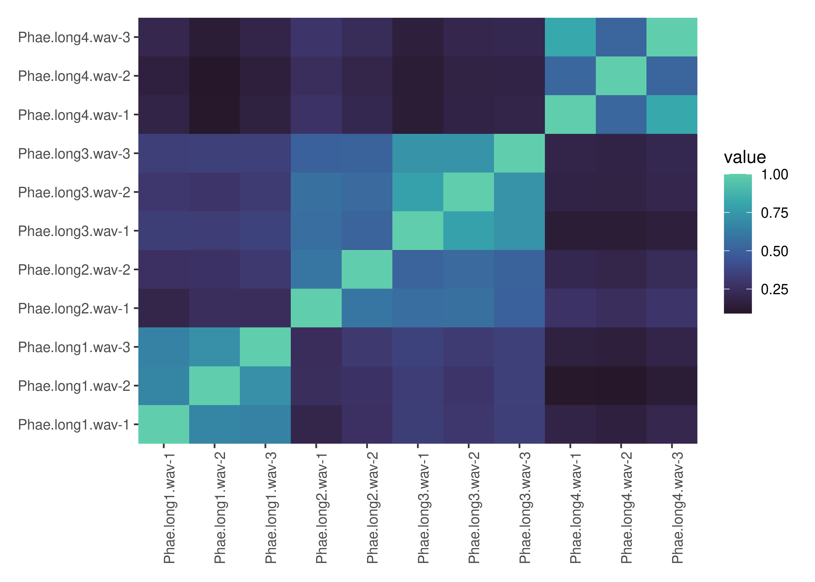

The acoustic space defined by the pairwise similarities can be projected into two axis using multidimensional scaling:

# convert into distances
xcor_dist <- 1 - xcor

# multidimensional scaling
mds <- cmdscale(xcor_dist, k = 2)

# extract first 2 vectors
xcor_mds <- data.frame(lbh_selec_table[, 1:2], mds = mds[, 1:2])

# print
xcor_mds

sound.files	channel	mds.1	mds.2
Phae.long1.wav	1	-0.1709890	-0.3935747
Phae.long1.wav	1	-0.2705734	-0.3811362
Phae.long1.wav	1	-0.2060406	-0.3615014
Phae.long2.wav	1	-0.0357237	0.3068145
Phae.long2.wav	1	-0.1165148	0.2365544
Phae.long3.wav	1	-0.2749377	0.2242787
Phae.long3.wav	1	-0.2081367	0.2673117
Phae.long3.wav	1	-0.2096715	0.1971588
Phae.long4.wav	1	0.5201505	-0.0307725
Phae.long4.wav	1	0.4828695	-0.0221744
Phae.long4.wav	1	0.4895673	-0.0429590

Note that the correlations are converted into distance by subtracting them from 1. This simplified acoustic space can also be easily visualized with a scatterplot:

ggplot(xcor_mds,
       aes(
         x = mds.1,
         y = mds.2,
         color = sound.files,
         shape =  sound.files
       )) +
  geom_point(size = 5) +
  scale_color_viridis_d(option = "G",
                        end = 0.9,
                        direction = -1) +
  theme_classic() +
  labs(x = "MDS1", y = "MDS2") +
  theme(legend.position = "right")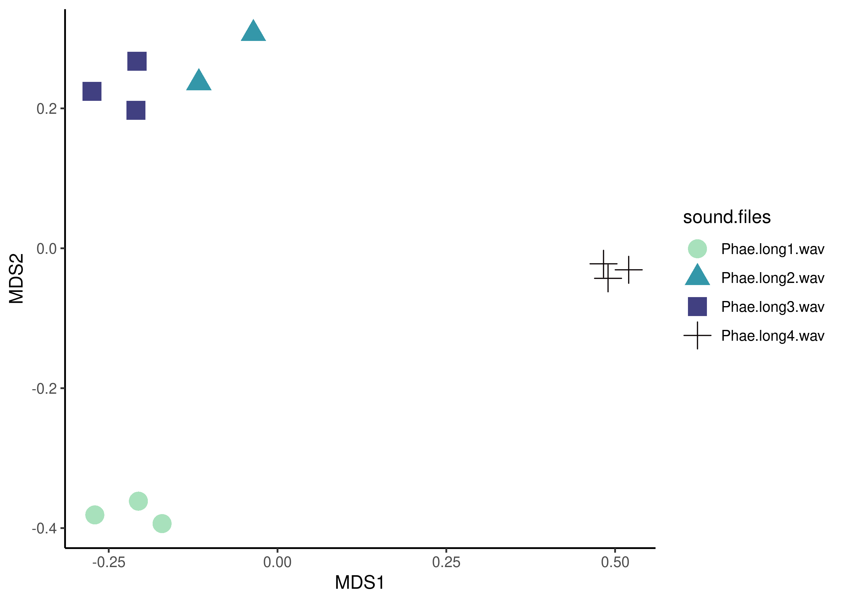

Exercise

• What does the argument type do and how does it affect the performance of the function?

• What does the pb argument do?

4 Dynamic time warping

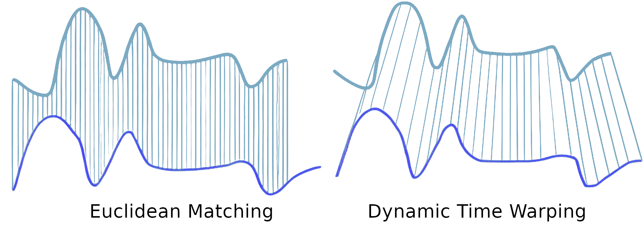
In time series analysis, time dynamics distortion (DTW) is one of the algorithms to measure the similarity between two time sequences, which may vary in their ‘speed’. The sequences are nonlinearly ‘warped’ in the temporal dimension to determine a measure of their similarity independent of certain nonlinear variations in the temporal dimension.

The freq_DTW() function extracts the dominant frequency values as a time series and then calculates the acoustic dissimilarity using dynamic time warping. The function uses the approx() function to interpolate values between the dominant frequency measurements:

dtw_dist <- freq_DTW(lbh_selec_table)

	Phae.long1.wav-1	Phae.long1.wav-2	Phae.long1.wav-3	Phae.long2.wav-1	Phae.long2.wav-2	Phae.long3.wav-1	Phae.long3.wav-2	Phae.long3.wav-3	Phae.long4.wav-1	Phae.long4.wav-2	Phae.long4.wav-3
Phae.long1.wav-1	0.0000	12.1613	27.2602	18.7335	21.1790	20.6645	18.9116	24.5375	25.1648	26.0236	22.7189
Phae.long1.wav-2	12.1613	0.0000	18.5390	15.8735	20.2081	17.6739	18.1535	24.4244	26.3725	27.7397	24.8443
Phae.long1.wav-3	27.2602	18.5390	0.0000	29.5158	29.0963	24.9517	28.4032	28.1725	31.7433	33.2878	31.1858
Phae.long2.wav-1	18.7335	15.8735	29.5158	0.0000	14.3232	13.8198	12.7713	17.9298	20.9547	19.6867	20.0898
Phae.long2.wav-2	21.1790	20.2081	29.0963	14.3232	0.0000	11.3861	8.1233	11.0131	25.7860	23.6662	22.5058
Phae.long3.wav-1	20.6645	17.6739	24.9517	13.8198	11.3861	0.0000	7.0170	9.9718	28.4507	31.6782	26.2246
Phae.long3.wav-2	18.9116	18.1535	28.4032	12.7713	8.1233	7.0170	0.0000	8.0238	24.8983	26.0703	23.6189
Phae.long3.wav-3	24.5375	24.4244	28.1725	17.9298	11.0131	9.9718	8.0238	0.0000	31.0330	32.2880	28.7885
Phae.long4.wav-1	25.1648	26.3725	31.7433	20.9547	25.7860	28.4507	24.8983	31.0330	0.0000	10.2553	3.6062
Phae.long4.wav-2	26.0236	27.7397	33.2878	19.6867	23.6662	31.6782	26.0703	32.2880	10.2553	0.0000	8.3373
Phae.long4.wav-3	22.7189	24.8443	31.1858	20.0898	22.5058	26.2246	23.6189	28.7885	3.6062	8.3373	0.0000

The function returns a matrix with paired dissimilarity values.

If img = TRUE, the function also produces image files with the spectrograms of the signals listed in the input data frame that shows the location of the dominant frequencies.

freq_DTW(
  lbh_selec_table,
  img = TRUE,
  col = "red",
  pch = 21,
  line = FALSE
)

 

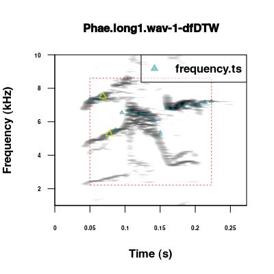
Frequency contours can be calculated independently using the freq_ts() function. These contours can be adjusted manually with the tailor_sels() function.

The DTW distance matrix returned by the function can also be visualized as a heatmap:

# present xcor as a heatmap using ggplot2
ggheatmap(dtw_dist) +
  scale_fill_viridis_c(
    option = "G",
    direction = -1,
    begin = 0.1,
    end = 0.8
  ) +
  theme(axis.text.x = element_text(angle = 90))

→ heatmap built with `geom_tile()`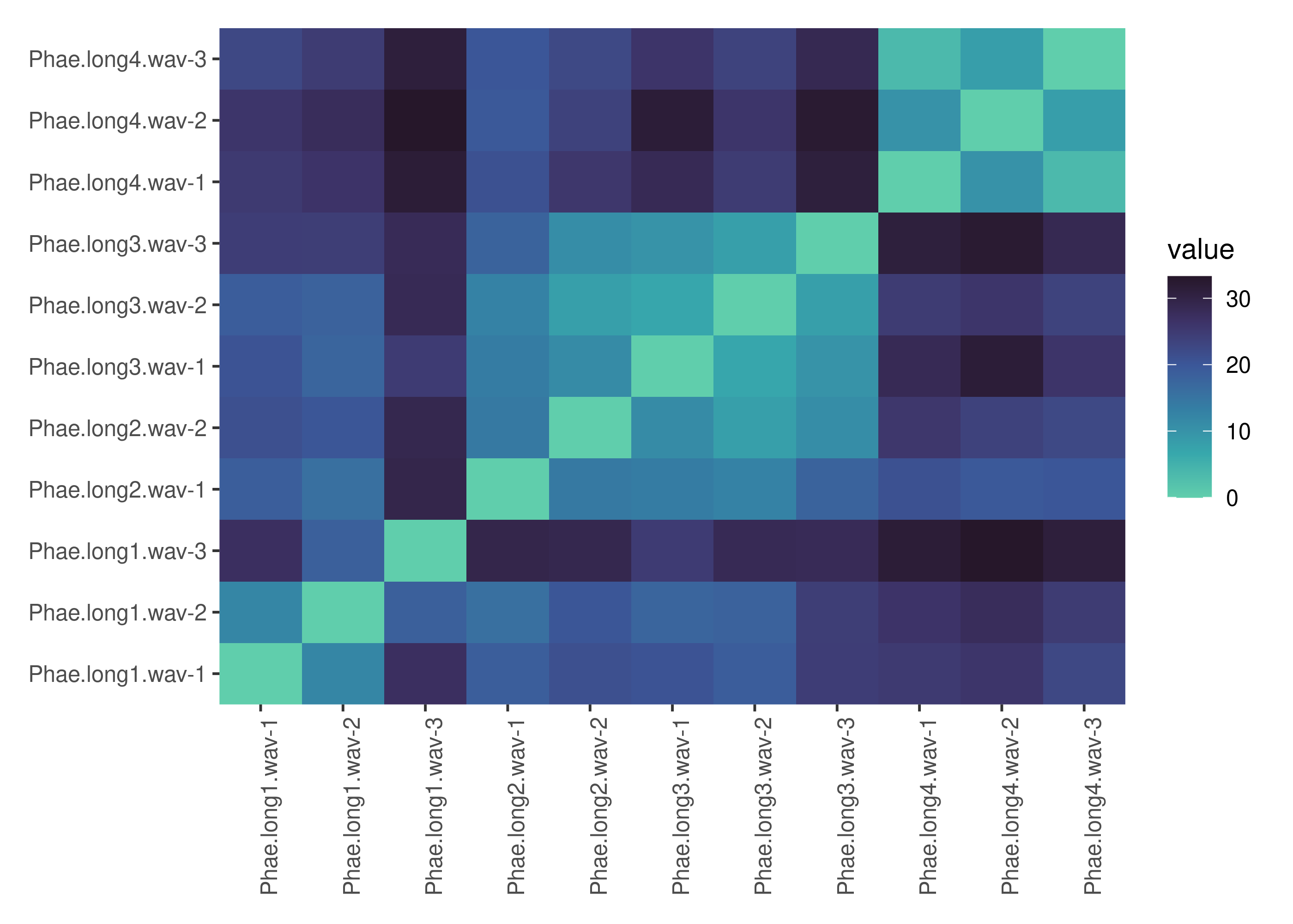

Similar to cross-correlation, the acoustic space defined by the pairwise DTW distances can be projected into two axis using multidimensional scaling:

# multidimensional scaling
mds <- cmdscale(dtw_dist, k = 2)

# extract first 2 vectors
dtw_mds <- data.frame(lbh_selec_table[, 1:2], mds = mds[, 1:2])

# print
dtw_mds

sound.files	selec	mds.1	mds.2
Phae.long1.wav	1	-1.3690867	-4.6219220
Phae.long1.wav	2	-5.0479486	-9.7416612
Phae.long1.wav	3	-6.9214972	-19.5585895
Phae.long2.wav	1	-0.1270242	5.0148052
Phae.long2.wav	2	-5.0891583	7.9875667
Phae.long3.wav	1	-11.5653234	3.4680210
Phae.long3.wav	2	-6.9615447	7.0664266
Phae.long3.wav	3	-12.5624223	8.0038274
Phae.long4.wav	1	16.6743151	-0.0970060
Phae.long4.wav	2	18.0756225	1.5591853
Phae.long4.wav	3	14.8940678	0.9193464

And again, this simplified acoustic space can be easily visualized with a scatterplot:

ggplot(dtw_mds,
       aes(
         x = mds.1,
         y = mds.2,
         color = sound.files,
         shape =  sound.files
       )) +
  geom_point(size = 5) +
  scale_color_viridis_d(option = "G",
                        end = 0.9,
                        direction = -1) +
  theme_classic() +
  labs(x = "MDS1", y = "MDS2") +
  theme(legend.position = "right")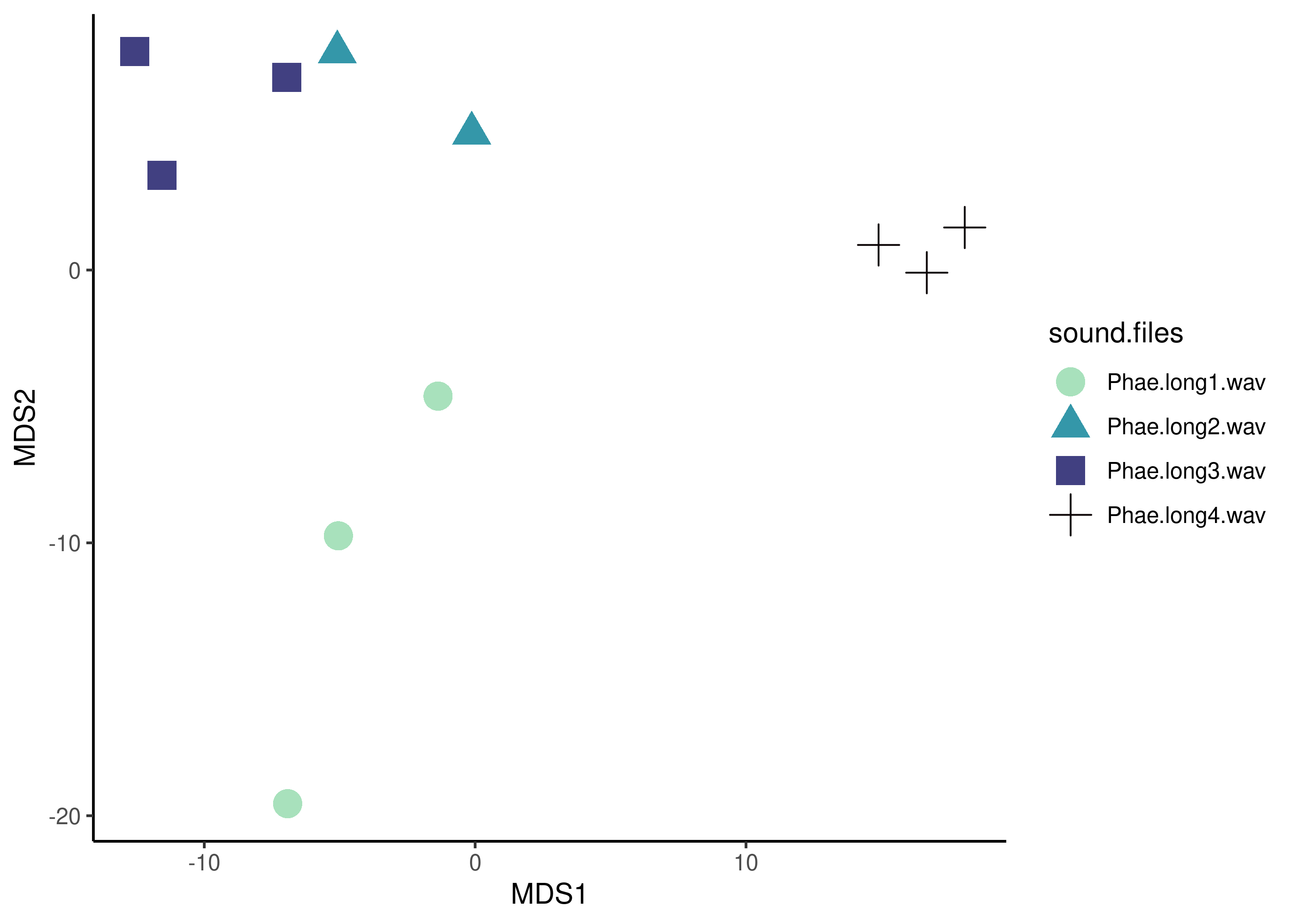

Exercise

 

• What do the length.out argument infreq_DTW()?

• Calculate spectrographic cross-correlation for the inquiry calls from these individuals: c("206433", "279470", "279533", "279820"). The extended selection table can be downloaded and read as follows:

download.file(url = "https://ndownloader.figshare.com/files/21167052", 
 destfile = "./examples/iniquiry_calls.RDS")

iniquiry_calls <- readRDS("./examples/iniquiry_calls.RDS")

• We can use a binary matrix to represent call membership. It has to be a pairwise matrix in which 0 denotes pairs of calls that belong to the same individual and 1 pairs that belong to different individuals. The function binary_triangular_matrix from the package PhenotypeSpace creates this type of matrix for representing call membership at the individual level:

bi_mat <- binary_triangular_matrix(iniquiry_calls$indiv)

Compare dissimilarity from cross-correlation (1 - correlation matrix) with individual call membership matrix using Mantel test (you can use vegan::mantel())

 

• Do the same test but this time using cepstral coefficient cross-correlation (hint: see argument “type”)

• Do the same test using dynamic time warping distances

 

5 Additional measures

5.1 Signal-to-noise ratio

sig2noise() measures this parameter. The duration of the margin in which to measure the background noise must be provided (mar argument):

snr <- sig2noise(X = lbh_selec_table, mar = 0.06)

snr

sound.files	channel	selec	start	end	bottom.freq	top.freq	SNR
Phae.long1.wav	1	1	1.1693549	1.3423884	2.220105	8.604378	21.88086
Phae.long1.wav	1	2	2.1584085	2.3214565	2.169437	8.807053	21.17991
Phae.long1.wav	1	3	0.3433366	0.5182553	2.218294	8.756604	19.79567
Phae.long2.wav	1	1	0.1595983	0.2921692	2.316862	8.822316	23.60318
Phae.long2.wav	1	2	1.4570585	1.5832087	2.284006	8.888027	26.99167
Phae.long3.wav	1	1	0.6265520	0.7577715	3.006834	8.822316	25.80051
Phae.long3.wav	1	2	1.9742132	2.1043921	2.776843	8.888027	26.05994
Phae.long3.wav	1	3	0.1233643	0.2545812	2.316862	9.315153	24.61822
Phae.long4.wav	1	1	1.5168116	1.6622365	2.513997	9.216586	28.15947
Phae.long4.wav	1	2	2.9326920	3.0768784	2.579708	10.235116	29.30194
Phae.long4.wav	1	3	0.1453977	0.2904966	2.579708	9.742279	24.75542

 

5.2 Inflections

Inflections in this case are defined as changes in the slope of a frequency contour. They can be used as a measure of frequency modulation. They can be calculated using the inflections() function on previously measured frequency contours:

cntrs <- freq_ts(X = lbh_selec_table)

inflcts <- inflections(cntrs)

sound.files	selec	inflections
Phae.long1.wav	1	9
Phae.long1.wav	2	10
Phae.long1.wav	3	8
Phae.long2.wav	1	13
Phae.long2.wav	2	9
Phae.long3.wav	1	11
Phae.long3.wav	2	8
Phae.long3.wav	3	10
Phae.long4.wav	1	5
Phae.long4.wav	2	5
Phae.long4.wav	3	5

 

5.3 Features at higher levels of organization

Vocalizations can be organized above the basic signal units like in long repertoire songs or multi-syllable calls. For instance, the song of the scale-throated hermit (Phaethornis eurynome) its composed of two elements:

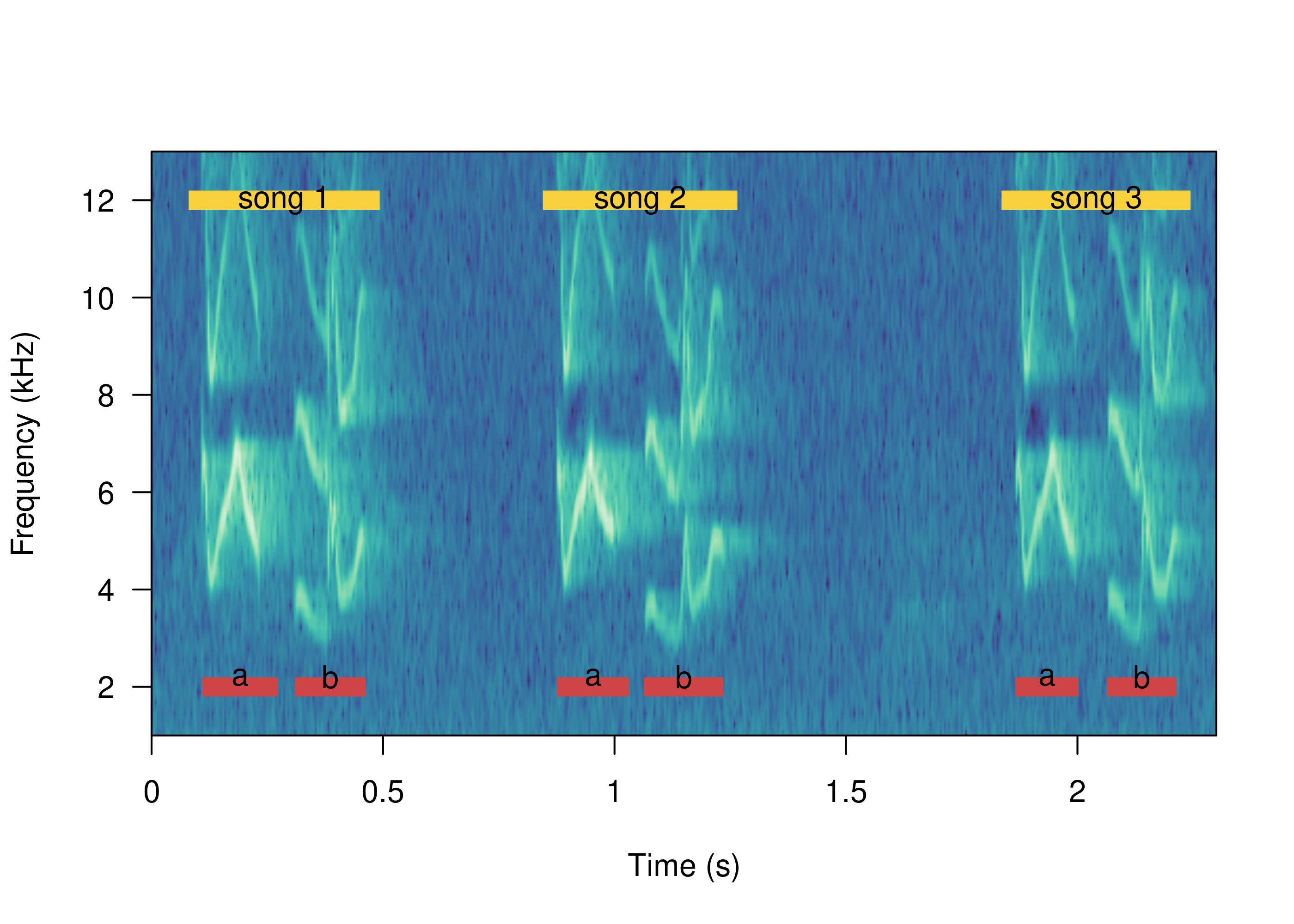
In cases like this we often want to describe the structure at the song level, rather than at the element level. We can do this using the function song_analysis(). By the default the function computes several metrics characterizing the structure of this higher levels of organization:

# read extended selection table
sth_est <- readRDS(file = "./examples/pha_eur_est.RDS")

# measure default features
song_analysis(
  X = sth_est,
  song_colm = "song",
  parallel = 1,
  pb = TRUE
)

sound.files	selec	start	end	top.freq	bottom.freq	song	Channel	num.elms	elm.duration	freq.range	song.duration	song.rate	gap.duration
Phaethornis-eurynome-15607.wav-song_1	1	0.1	0.478118	9.15075	2.97675	1	1	2	0.176644	6.17400	0.378118	9.86135	0.024830
Phaethornis-eurynome-15607.wav-song_2	1	0.1	0.476894	10.00000	2.97675	2	1	2	0.176055	7.02325	0.376894	9.95148	0.024785
Phaethornis-eurynome-15607.wav-song_3	1	0.1	0.471089	10.00000	3.19725	3	1	2	0.176157	6.80275	0.371089	10.01134	0.018776
Phaethornis-eurynome-15607.wav-song_4	1	0.1	0.478322	9.81225	3.19725	4	1	2	0.182903	6.61500	0.378322	10.66376	0.012517

We can also compute average or extreme values of acoustic features. This can be done on element-level features extracted with other functions:

# measure acoustic features
sp <- spectro_analysis(sth_est, bp = c(1, 11), 300, fast = TRUE)

sp <- merge(sp, sth_est, by = c("sound.files", "selec"))

# caculate song-level features for all numeric features
song_analysis(
  X = sp,
  song_colm = "song",
  parallel = 1,
  pb = TRUE
)

sound.files	selec	start	end	top.freq	bottom.freq	song	duration	meanfreq	sd	freq.median	freq.Q25	freq.Q75	freq.IQR	time.median	time.Q25	time.Q75	time.IQR	peakt	skew	kurt	sp.ent	time.ent	entropy	sfm	meandom	mindom	maxdom	dfrange	modindx	startdom	enddom	dfslope	meanpeakf	Channel	num.elms	elm.duration	freq.range	song.duration	song.rate	gap.duration
Phaethornis-eurynome-15607.wav-song_1	1	0.1	0.478118	9.15075	2.97675	1	0.176644	6.26096	1.68862	5.92027	5.13720	7.14686	2.00966	0.088325	0.050015	0.118474	0.068459	0.111375	2.78389	14.03501	0.888248	0.886249	0.787229	0.303150	5.89941	1.617	8.8200	7.2030	5.75042	3.8955	5.8800	11.421040	6.3945	1	2	0.176644	6.17400	0.378118	9.86135	0.024830
Phaethornis-eurynome-15607.wav-song_2	1	0.1	0.476894	10.00000	2.97675	2	0.176055	6.34424	1.73260	6.00156	5.15780	7.33125	2.17345	0.087856	0.049598	0.120447	0.070849	0.062043	2.70287	13.59398	0.892654	0.886421	0.791280	0.325522	6.12504	3.969	8.9670	4.9980	9.48831	5.1450	5.1450	0.004517	5.7330	1	2	0.176055	7.02325	0.376894	9.95148	0.024785
Phaethornis-eurynome-15607.wav-song_3	1	0.1	0.471089	10.00000	3.19725	3	0.176157	6.38094	1.70429	6.11488	5.20910	7.37644	2.16734	0.090052	0.053541	0.118759	0.065218	0.092544	2.45565	10.27109	0.889185	0.886213	0.788051	0.313459	5.93620	2.793	9.3345	6.5415	11.07233	5.0715	5.9535	4.827083	7.0560	1	2	0.176157	6.80275	0.371089	10.01134	0.018776
Phaethornis-eurynome-15607.wav-song_4	1	0.1	0.478322	9.81225	3.19725	4	0.182903	6.43292	1.68863	6.45064	5.17807	7.32800	2.14993	0.089847	0.048813	0.122748	0.073935	0.090210	2.29066	9.58674	0.880072	0.885443	0.779209	0.301317	6.05304	4.263	8.9670	4.7040	5.45294	6.6150	5.1450	-7.878768	6.4680	1	2	0.182903	6.61500	0.378322	10.66376	0.012517

 

We can also compute song-level features selecting features with ‘mean_colm’:

# caculate song-level features selecting features with mean_colm
song_analysis(
  X = sp,
  song_colm = "song",
  mean_colm = c("dfrange", "duration"),
  parallel = 1,
  pb = TRUE
)

sound.files	selec	start	end	top.freq	bottom.freq	song	dfrange	duration	num.elms	elm.duration	freq.range	song.duration	song.rate	gap.duration
Phaethornis-eurynome-15607.wav-song_1	1	0.1	0.478118	9.15075	2.97675	1	7.2030	0.176644	2	0.176644	6.17400	0.378118	9.86135	0.024830
Phaethornis-eurynome-15607.wav-song_2	1	0.1	0.476894	10.00000	2.97675	2	4.9980	0.176055	2	0.176055	7.02325	0.376894	9.95148	0.024785
Phaethornis-eurynome-15607.wav-song_3	1	0.1	0.471089	10.00000	3.19725	3	6.5415	0.176157	2	0.176157	6.80275	0.371089	10.01134	0.018776
Phaethornis-eurynome-15607.wav-song_4	1	0.1	0.478322	9.81225	3.19725	4	4.7040	0.182903	2	0.182903	6.61500	0.378322	10.66376	0.012517

 

.. and compute song-level features for selecting features with ‘mean_colm’, ‘max_colm’ and ‘min_colm’ and weighted by duration:

song_analysis(
  X = sp,
  weight = "duration",
  song_colm = "song",
  mean_colm =  c("dfrange", "duration"),
  min_colm =  "mindom",
  max_colm = "maxdom",
  parallel = 1,
  pb = TRUE
)

sound.files	selec	start	end	top.freq	bottom.freq	song	dfrange	duration	min.mindom	max.maxdom	num.elms	elm.duration	freq.range	song.duration	song.rate	gap.duration
Phaethornis-eurynome-15607.wav-song_1	1	0.1	0.478118	9.15075	2.97675	1	7.19966	0.176654	1.1025	8.8935	2	0.176644	6.17400	0.378118	9.86135	0.024830
Phaethornis-eurynome-15607.wav-song_2	1	0.1	0.476894	10.00000	2.97675	2	4.99789	0.176055	3.7485	9.0405	2	0.176055	7.02325	0.376894	9.95148	0.024785
Phaethornis-eurynome-15607.wav-song_3	1	0.1	0.471089	10.00000	3.19725	3	6.57584	0.176290	2.1315	9.9225	2	0.176157	6.80275	0.371089	10.01134	0.018776
Phaethornis-eurynome-15607.wav-song_4	1	0.1	0.478322	9.81225	3.19725	4	4.71665	0.183241	3.8955	9.0405	2	0.182903	6.61500	0.378322	10.66376	0.012517

 

 

Exercise

 

• Spix’s disc-winged bats (Thyroptera tricolor) its a Neotropical species that uses a specific call type to reply to social mates looking for their roosts. Those ‘response’ calls look like this:

 

 

An extended selection table with response calls can be read from github as follows:

download.file(url = "https://github.com/maRce10/OTS_BIR_2025/raw/master/examples/response_calls.RDS", 
 destfile = "./examples/response_calls.RDS")

response_calls <- readRDS("./examples/response_calls.RDS")

 

• Calculate spectrographic features (spectro_analysis()) for the Spix’s disc-winged bat response calls.

• Summarize features by call (song_analysis()). To do that you should add the column ‘start’, ‘end’ and ‘call’ to the output of spectro_analysis()

 

---

6 References

1. Araya-Salas M, A Hernández-Pinsón N Rojas, G Chaverri. (2020). Ontogeny of an interactive call-and-response system in Spix’s disc-winged bats. Animal Behaviour.

2. Araya-Salas M, Smith-Vidaurre G (2017) warbleR: An R package to streamline analysis of animal acoustic signals. Methods Ecol Evol 8:184–191.

3. Lyon, R. H., & Ordubadi, A. (1982). Use of cepstra in acoustical signal analysis. Journal of Mechanical Design, 104(2), 303-306.

4. Salamon, J., Jacoby, C., & Bello, J. P. (2014). A dataset and taxonomy for urban sound research. In Proceedings of the 22nd ACM international conference on Multimedi. 1041-1044.

Session information

R version 4.5.0 (2025-04-11)
Platform: x86_64-pc-linux-gnu
Running under: Ubuntu 22.04.5 LTS

Matrix products: default
BLAS:   /usr/lib/x86_64-linux-gnu/blas/libblas.so.3.10.0 
LAPACK: /usr/lib/x86_64-linux-gnu/lapack/liblapack.so.3.10.0  LAPACK version 3.10.0

locale:
 [1] LC_CTYPE=en_US.UTF-8       LC_NUMERIC=C              
 [3] LC_TIME=es_CR.UTF-8        LC_COLLATE=en_US.UTF-8    
 [5] LC_MONETARY=es_CR.UTF-8    LC_MESSAGES=en_US.UTF-8   
 [7] LC_PAPER=es_CR.UTF-8       LC_NAME=C                 
 [9] LC_ADDRESS=C               LC_TELEPHONE=C            
[11] LC_MEASUREMENT=es_CR.UTF-8 LC_IDENTIFICATION=C       

time zone: America/Costa_Rica
tzcode source: system (glibc)

attached base packages:
[1] stats     graphics  grDevices utils     datasets  methods   base     

other attached packages:
 [1] Rraven_1.0.14        PhenotypeSpace_0.1.0 ggalign_1.0.1       
 [4] ggplot2_3.5.2        viridis_0.6.5        viridisLite_0.4.2   
 [7] kableExtra_1.4.0     warbleR_1.1.35       NatureSounds_1.0.5  
[10] knitr_1.50           seewave_2.2.3        tuneR_1.4.7         

loaded via a namespace (and not attached):
 [1] tidyselect_1.2.1       dplyr_1.1.4            farver_2.1.2          
 [4] bitops_1.0-9           fastmap_1.2.0          RCurl_1.98-1.17       
 [7] spatstat.geom_3.3-6    spatstat.explore_3.4-2 digest_0.6.37         
[10] lifecycle_1.0.4        Deriv_4.1.6            cluster_2.1.8.1       
[13] sf_1.0-20              spatstat.data_3.1-6    terra_1.8-42          
[16] magrittr_2.0.3         compiler_4.5.0         rlang_1.1.6           
[19] tools_4.5.0            yaml_2.3.10            labeling_0.4.3        
[22] htmlwidgets_1.5.4      sp_2.2-0               classInt_0.4-11       
[25] curl_6.2.2             xml2_1.3.8             RColorBrewer_1.1-3    
[28] abind_1.4-8            KernSmooth_2.23-26     withr_3.0.2           
[31] grid_4.5.0             polyclip_1.10-7        e1071_1.7-16          
[34] iterators_1.0.14       scales_1.4.0           MASS_7.3-65           
[37] spatstat.utils_3.1-3   signal_1.8-1           cli_3.6.5             
[40] vegan_2.6-10           rmarkdown_2.29         generics_0.1.3        
[43] rstudioapi_0.17.1      httr_1.4.7             rjson_0.2.23          
[46] DBI_1.2.3              pbapply_1.7-2          proxy_0.4-27          
[49] stringr_1.5.1          splines_4.5.0          fftw_1.0-9            
[52] parallel_4.5.0         Sim.DiffProc_4.9       vctrs_0.6.5           
[55] Matrix_1.7-3           jsonlite_2.0.0         tensor_1.5            
[58] systemfonts_1.2.3      foreach_1.5.2          testthat_3.2.3        
[61] spatstat.univar_3.1-2  shinyBS_0.61.1         units_0.8-7           
[64] goftest_1.2-3          glue_1.8.0             spatstat.random_3.3-3 
[67] dtw_1.23-1             codetools_0.2-20       stringi_1.8.7         
[70] gtable_0.3.6           deldir_2.0-4           raster_3.6-32         
[73] tibble_3.2.1           soundgen_2.7.2         pillar_1.10.2         
[76] htmltools_0.5.8.1      brio_1.1.5             R6_2.6.1              
[79] evaluate_1.0.3         lattice_0.22-7         class_7.3-23          
[82] Rcpp_1.0.14            permute_0.9-7          svglite_2.1.3         
[85] gridExtra_2.3          nlme_3.1-168           spatstat.sparse_3.1-0 
[88] mgcv_1.9-3             xfun_0.52              pkgconfig_2.0.3