Seewave

Published

May 17, 2025

Objectives

Understand the most common metrics of acoustic structure
Get familiar with manipulating and formatting sound in the R environment

seewave provides a wide variety of tools to accurately assess sound properties in the R environment. It is an extensive package with lots of features. The package allows to visualize and measure characteristics of time, frequency and amplitude of sounds. The tools are arranged in a modular way (each analysis in its own function) which allows combining them to generate more elaborate analyzes.

The majority of the functions of seewave work on wave objects (but not on audio files in folders). Here we will see examples of some of these tools, focusing on those that are potentially more useful for the study of vocal behavior in animals.

First we must load the package:

Code

library(seewave)

We can see the description of the package seewave in this way:

Code

?seewave

0.1 Example data in seewave

seewave brings several objects that we can use as an example to explore its functions. We can call them with the data () function:

Code

# cargar ejemplos
data(tico)

data(orni)

data(sheep)

⚠ data() only works to load examples that come with the packages by default, not to load your own audio files!!

We can see the information of each of them using ?:

Code

?tico

Exercise

What kind of object is tico?

What is the sampling rate and duration?

1 Oscillograms

You can create the oscillogram of the entire “wave” object like this:

Code

oscillo(tico)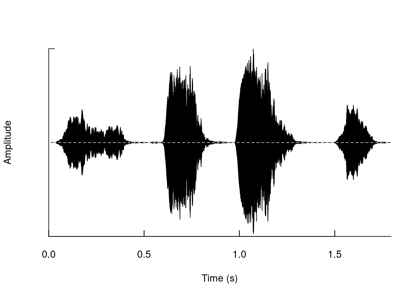

We can also generate it for a segment:

Code

oscillo(tico, from = 0, to = 1)

The visualizations in seewave allow a high degree of customization. For example change the color:

Code

oscillo(tico, from = 0, to = 1, colwave = "#8fcc78")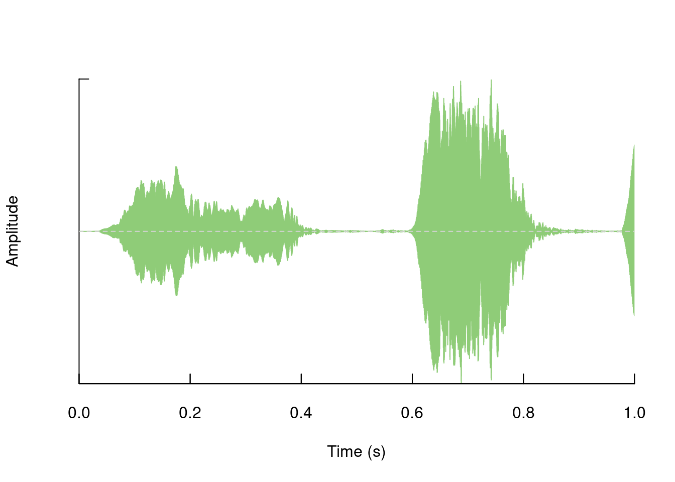

As with most seewave functions many other components of the chart can be modified, for example:

Code

# grey background
op <- par(bg = "grey")

oscillo(tico, f = 22050, k = 4 , j = 1,
        title = TRUE,
        colwave = "black", 
        coltitle = "yellow",
        collab = "red",
        colline = "white",
        colaxis = "blue",
        coly0 = "grey50")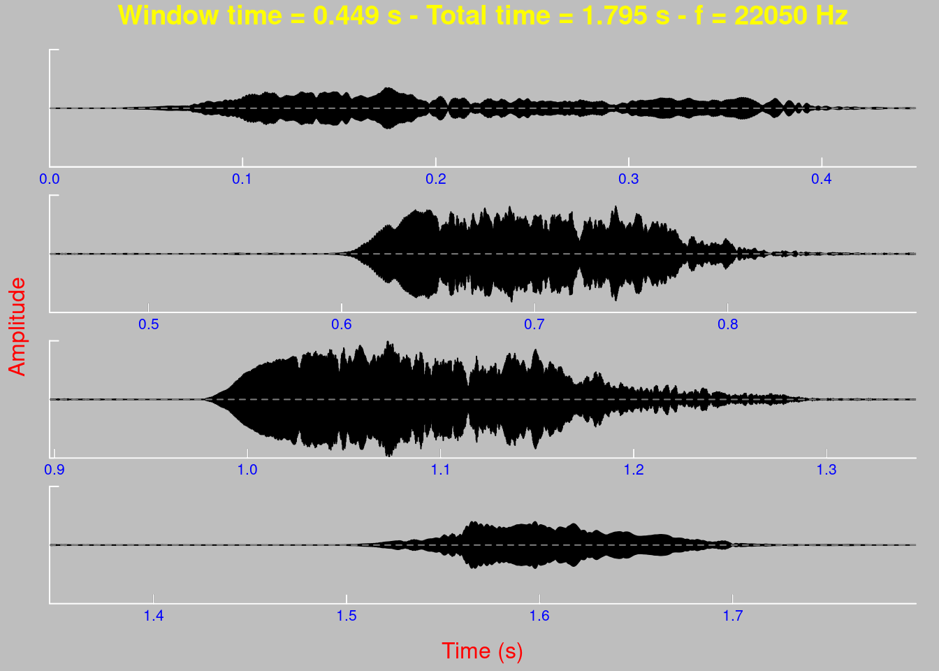

We can also generate other representations of “amplitude vs. time”, such as “amplitude envelopes”:

Code

env(tico, f = 22050, colwave = "#8fcc78")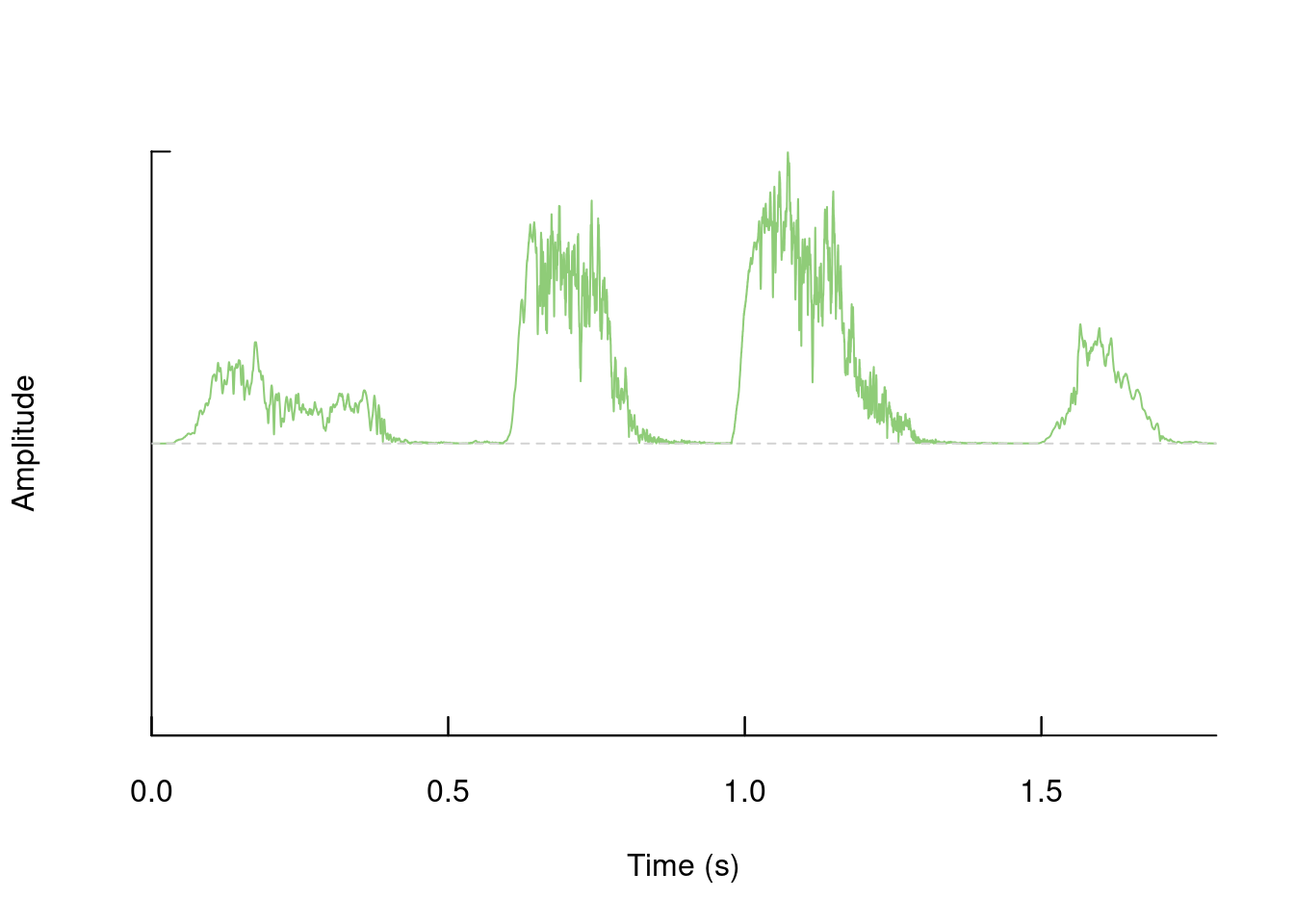

We can superimpose it on the oscillogram to facilitate comparison:

Code

oscillo(tico, f = 22050)

par(new=TRUE)

env(tico, f = 22050, colwave = "#8fcc78")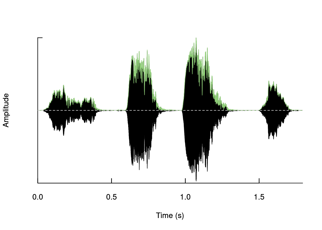

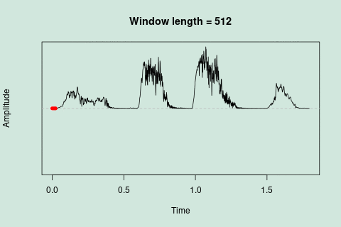
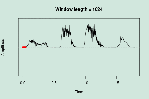
Sliding window for time series

Sliding windows allow you to smooth out the contours of a time series by calculating an average value around the “neighborhood” of values for a given value. In the case of amplitude envelope the size of the “neighborhood” is given by the length of the window (“wl”). The larger the window length, the greater the smoothing of the curve:

Sliding window

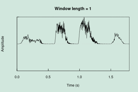
This animation shows how the amplitude envelope of the “tico” object is smoothed with a 512-point window:

Sliding window

… or a 1024 point window:

Sliding window

We can use these amplitude “hills” to define segments in the “wave” object using the timer() function. The “ssmooth” argument allows us to use a sliding window:

Code

tmr <- timer(orni, f = 22050, threshold = 5, ssmooth = 40, 
             bty = "l", colval = "#51c724")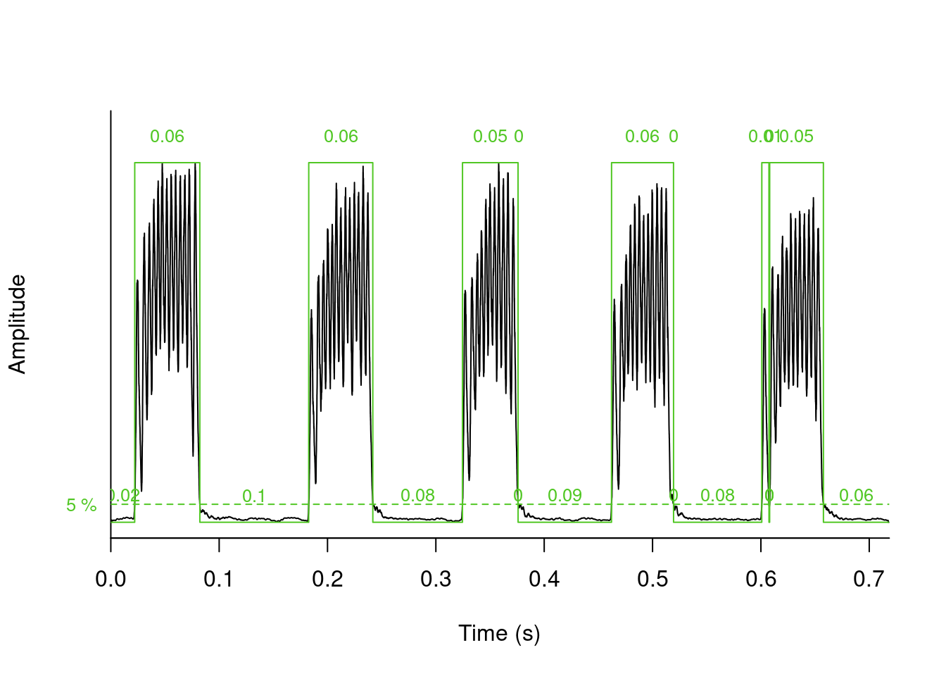

Code

tmr

$s
[1] 6.013985e-02 5.918741e-02 5.134111e-02 4.535434e-05 5.728253e-02
[6] 4.535434e-05 6.667088e-03 4.535434e-05 4.966300e-02

$p
 [1] 2.208756e-02 1.004599e-01 8.272631e-02 2.267717e-04 8.594647e-02
 [6] 4.535434e-05 8.132033e-02 4.988977e-04 4.535434e-05 6.068410e-02

$r
[1] 0.6552769

$s.start
[1] 0.02208756 0.18268727 0.32460099 0.37616887 0.46216069 0.51948857 0.60085425
[8] 0.60802024 0.60811095

$s.end
[1] 0.08222741 0.24187468 0.37594210 0.37621422 0.51944322 0.51953393 0.60752134
[8] 0.60806559 0.65777395

$first
[1] "pause"

The output is a list with the following elements:

s: duration of detected signals (in s)
p: duration of pauses (i.e. gaps) between signals
r: ratio of s to r
s.start: start of signals
end: end of signals

Exercise

In the previous example using timer() the last pulse is divided into 2 detections, one very small at the beginning and another containing the rest of the pulse. Change the “ssmooth” argument until this section is detected as a single pulse.

2 Power Spectra

We can visualize the amplitude in the frequency domain using power spectra. The meanspec() function calculates the average distribution of energy in the frequency range (the average power spectrum):

Code

mspc <- meanspec(orni, f = 22050, wl = 512, col = "#d1e7dd")

polygon(rbind(c(0, 0), mspc), col = "#d1e7dd")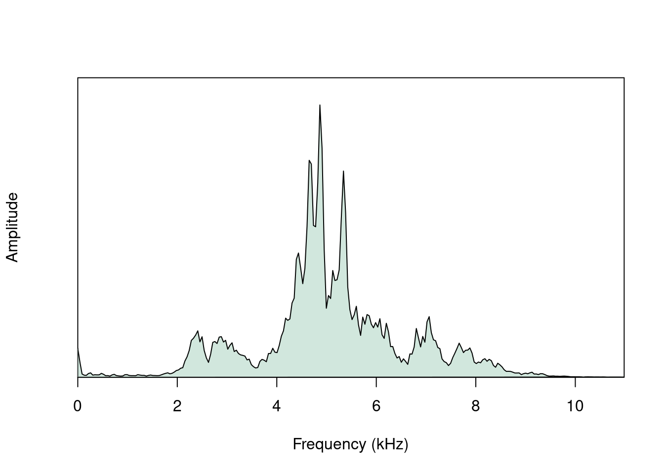

Code

nrow(mspc)

[1] 256

The spec() function, on the other hand, calculates the spectrum for the entire signal:

Code

spc <- spec(orni, f=22050, wl=512, col = "#8fcc78")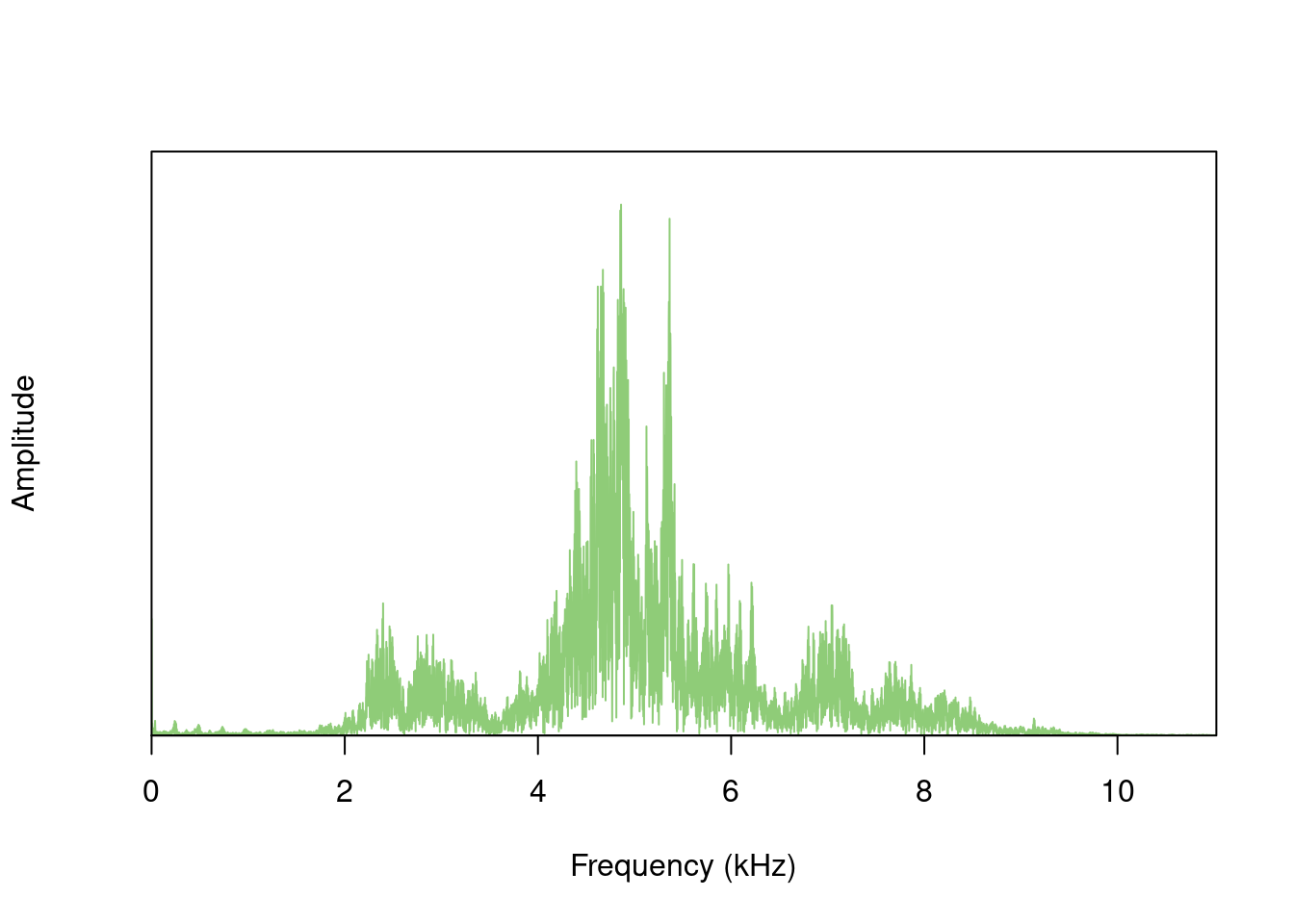

Code

nrow(spc)

[1] 7921

The result of spec() or meanspec() can be input into the fpeaks() function to calculate amplitude peaks:

Code

pks <- fpeaks(spc, nmax = 1)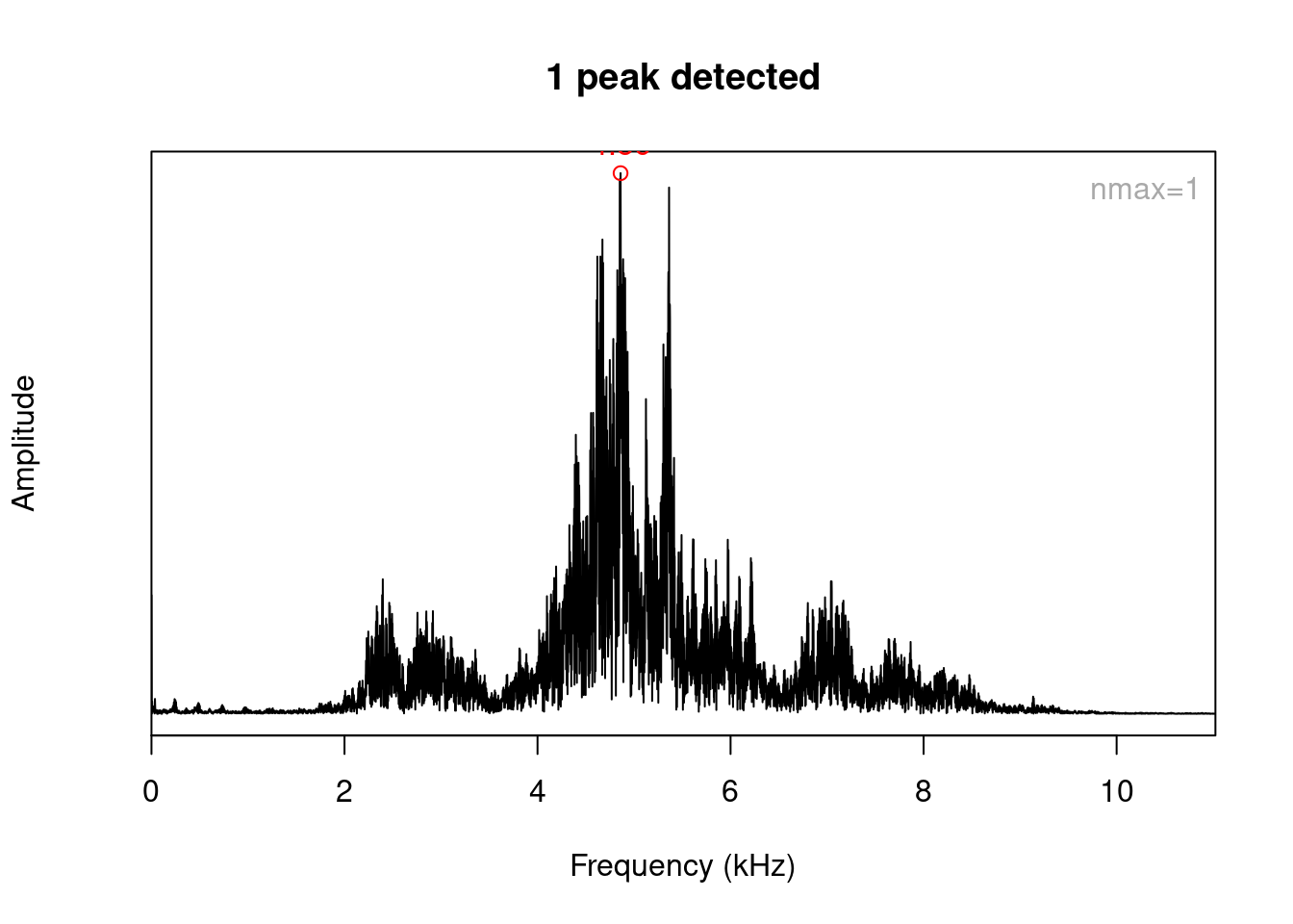

Code

pks

         [,1] [,2]
[1,] 4.860409    1

3 Wave manipulation

We can cut segments of a “wave” object:

Code

tico2 <- cutw(tico, to = 1, output = "Wave")

oscillo(tico2)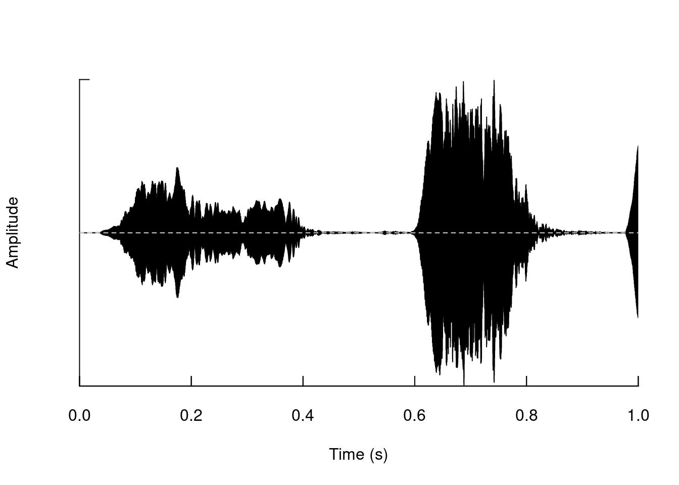

Add segments:

Code

tico3 <- pastew(tico, tico2, output = "Wave")

oscillo(tico3)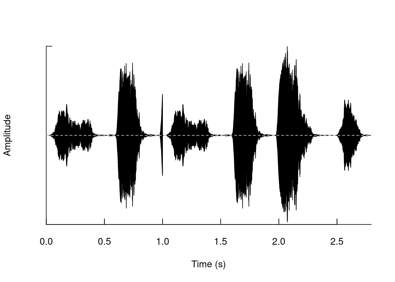

Remove segments:

Code

tico4 <- deletew(tico, output = "Wave", from = 0.55, to = 0.93)

oscillo(tico4)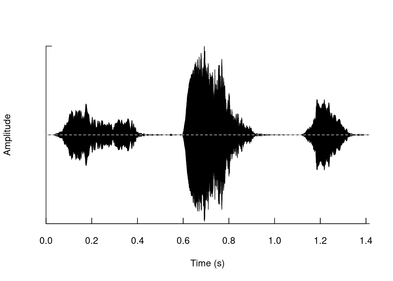

Add segments of silence:

Code

tico5 <- addsilw(tico, at = "end", d = 1, output = "Wave")

oscillo(tico5)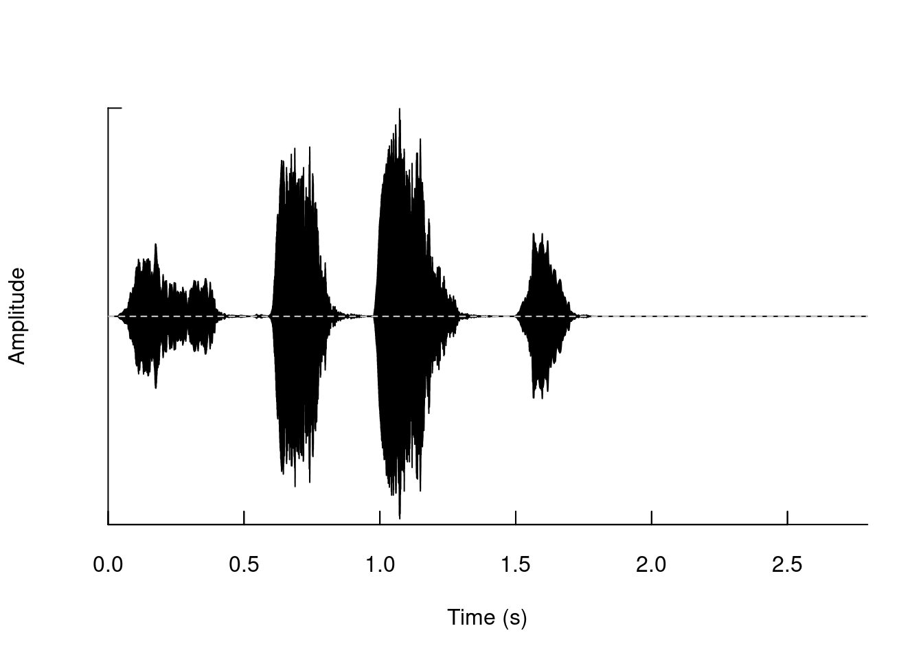

Code

duration(tico)

[1] 1.794921

Code

duration(tico5)

[1] 2.794921

Exercise

The function rev() can reverse the order of a vector:

Code

v1 <- c(1, 2, 3)

rev(v1)

[1] 3 2 1

Reverse the amplitude vector of ‘tico’ and generate a spectrogram of the reversed wave object

Filter out frequency bands:

Code

# original
spectro(tico, scale = FALSE, grid = FALSE, flim = c(2, 6))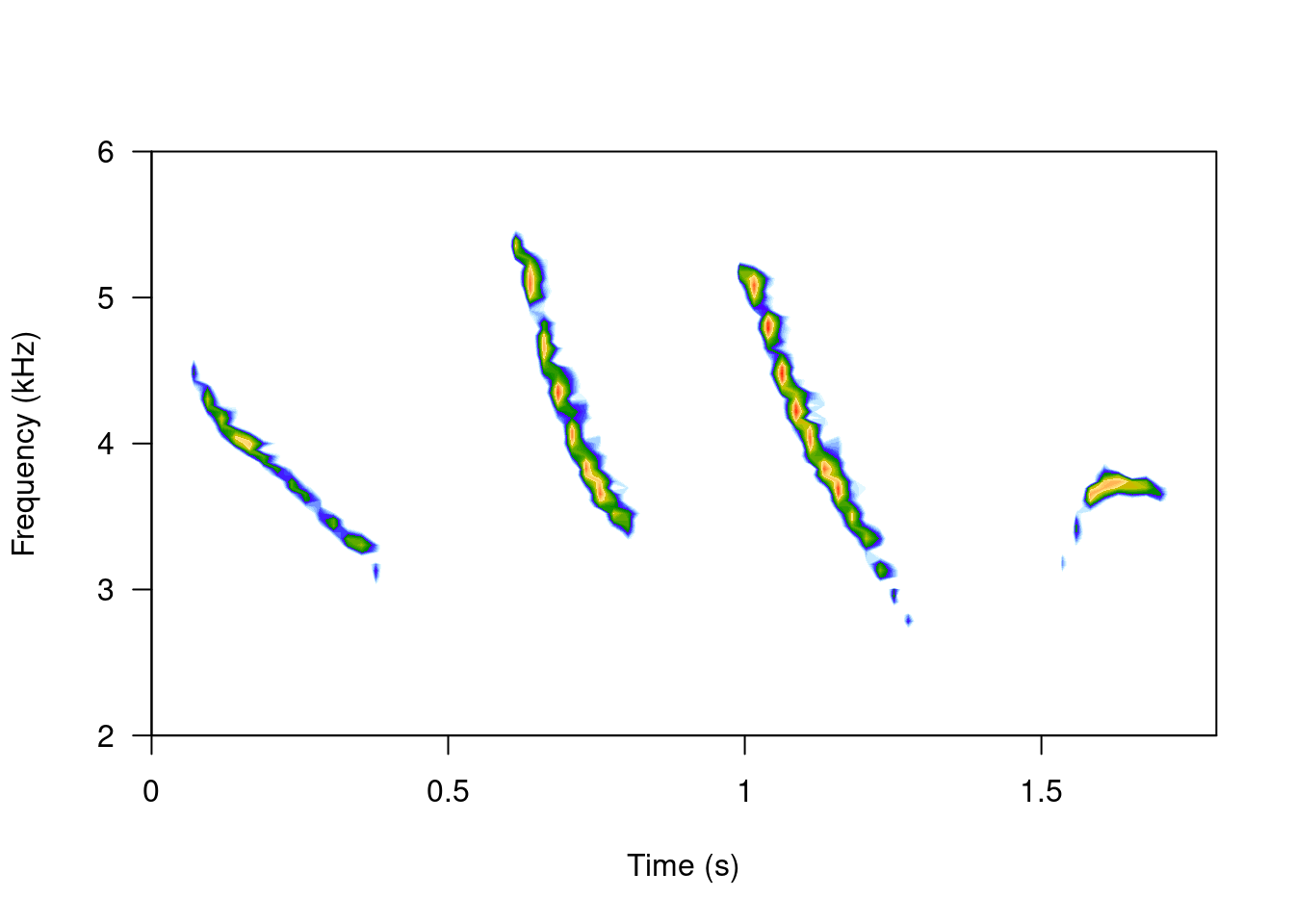

Code

# filtered
f_tico <- ffilter(tico, from = 4000, to = 6500, output = "Wave")

spectro(f_tico, scale = FALSE, grid = FALSE, flim = c(2, 6))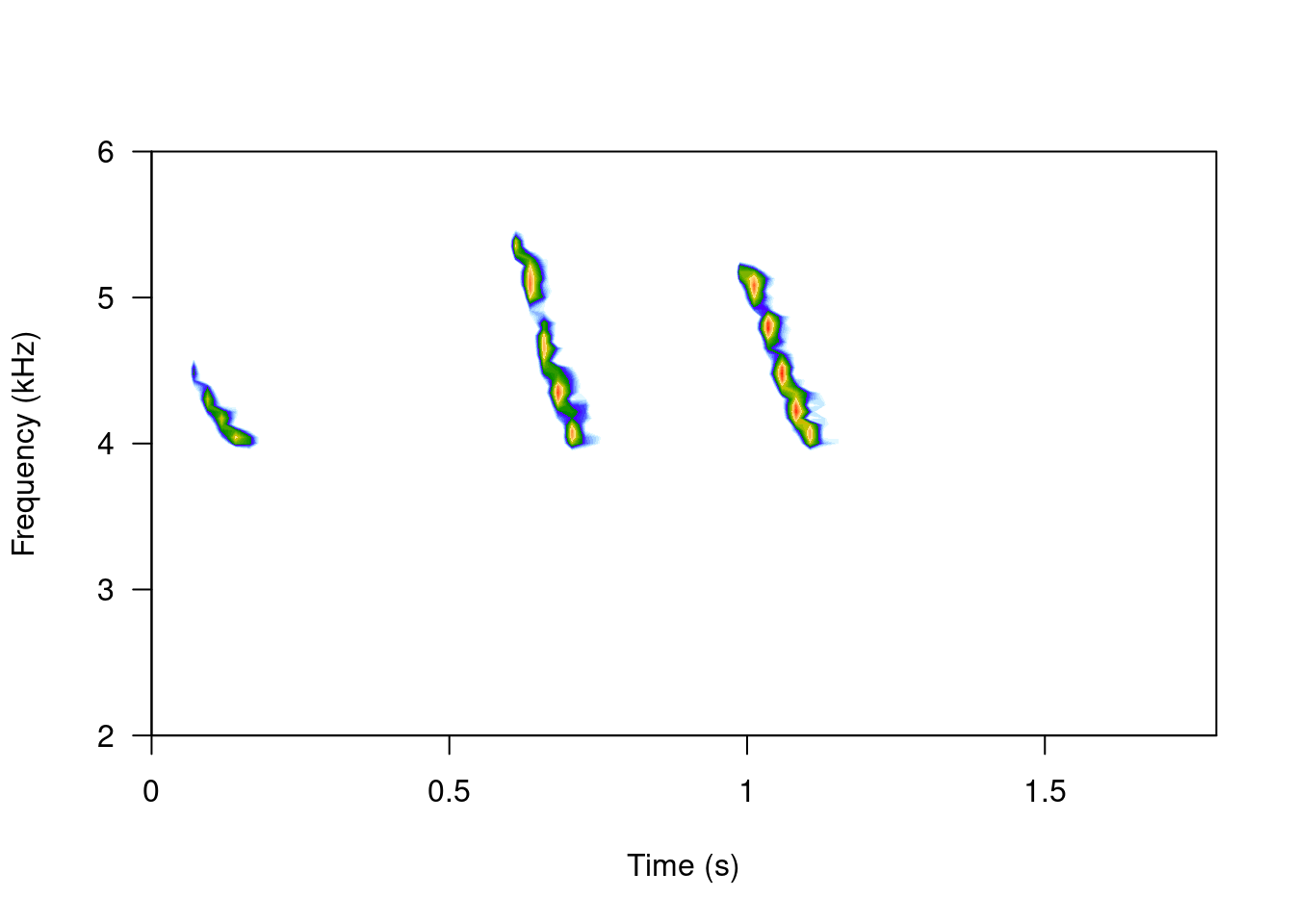

Change frequency (pitch):

Code

# cut the first
tico6 <- cutw(tico, from = 0, to = 0.5, output = "Wave")

# increase frec
tico.lfs <- lfs(tico6, shift = 1000, output = "Wave")

# decrease frec
tico.lfs.neg <- lfs(tico6, shift = -1000, output = "Wave")

# 3 column graph
opar <- par()
par(mfrow = c(1, 3))

# original
spectro(tico6, scale = FALSE, grid = FALSE, flim = c(1, 8), main = "original")

# modified
spectro(tico.lfs, scale = FALSE, grid = FALSE, flim = c(1, 8), main = "1 kHz up")

spectro(tico.lfs.neg, scale = FALSE, grid = FALSE, flim = c(1, 8), main = "1 kHz down")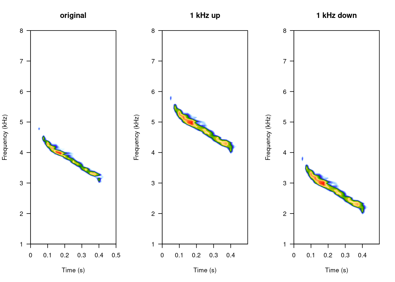

Code

par(opar)

4 Measurements

Apart from the measurements of peak frequency (fpeaks()) and duration (timer()), we can measure many other aspects of the acoustic signals using seewave. For example, we can estimate the fundamental frequency (which refers to the lowest frequency harmonic in the harmonic stack), with the fund() function:

Code

spectro(sheep, scale = FALSE, grid = FALSE)

par(new=TRUE)

ff <- fund(sheep, fmax = 300, ann = FALSE, threshold=6, col = "green")

Code

head(ff)

              x          y
[1,] 0.00000000         NA
[2,] 0.06677027         NA
[3,] 0.13354054         NA
[4,] 0.20031081         NA
[5,] 0.26708108 0.10000000
[6,] 0.33385135 0.07142857

This function uses cepstral transformation to detect the dominant frequency. The autoc() function also measures the fundamental frequency, only using autocorrelation.

Similarly we can measure the dominant frequency (the harmonic with the highest energy):

Code

par(new=TRUE)

df <- dfreq(sheep, f = 8000, fmax = 300, type = "p", pch = 24, ann = FALSE, threshold = 6, col = "red")

head(df)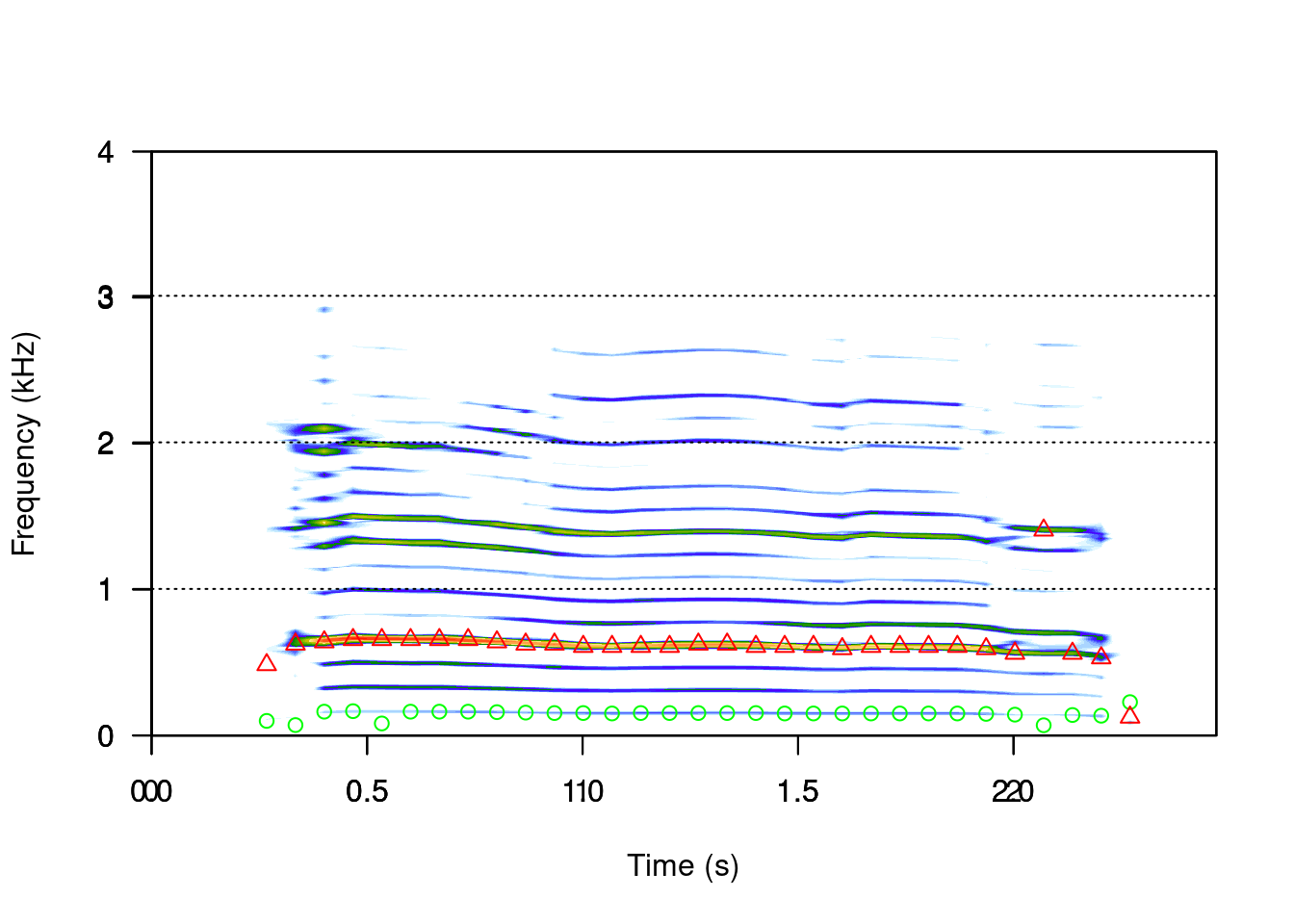

              x        y
[1,] 0.00000000       NA
[2,] 0.06677027       NA
[3,] 0.13354054       NA
[4,] 0.20031081       NA
[5,] 0.26708108 0.484375
[6,] 0.33385135 0.625000

Measure statistical descriptors of the amplitude distribution in frequency and time:

Code

# cut
note2 <- cutw(tico, from=0.6, to=0.9, output="Wave")

n2.as <- acoustat(note2)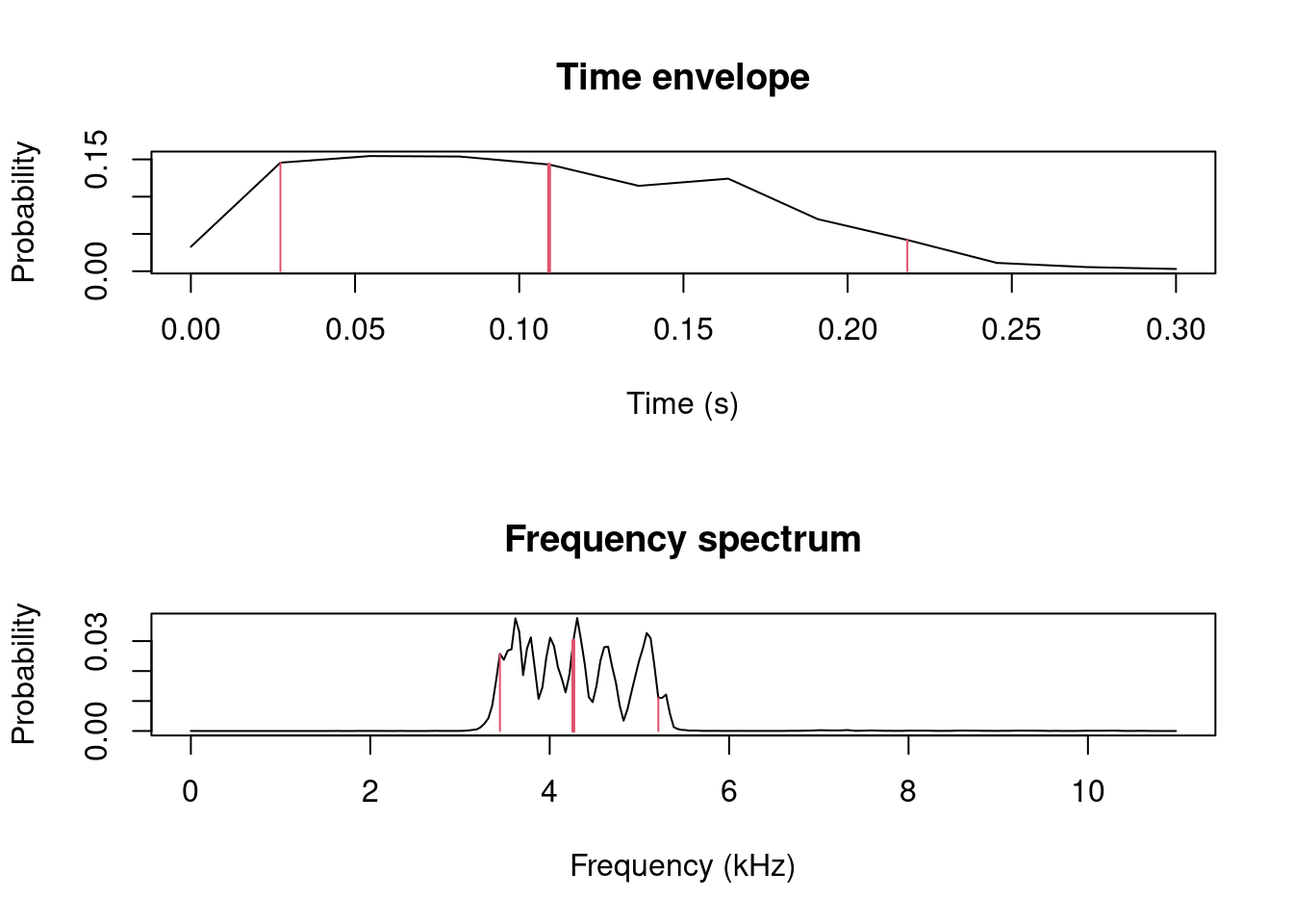

Code

as.data.frame(n2.as[3:8])

time.P1	time.M	time.P2	time.IPR	freq.P1	freq.M
0.0272727	0.1090909	0.2181818	0.1909091	3.445312	4.263574

Measure statistical descriptors of frequency spectra:

Code

# measure power spectrum
n2.sp <- meanspec(note2, plot = FALSE)

n2.spcp <- specprop(n2.sp, f = note2@samp.rate)

as.data.frame(n2.spcp)

mean	sd	median	sem	mode	Q25	Q75	IQR	cent	skewness	kurtosis	sfm	sh	prec
4346.889	694.2615	4306.641	43.39134	4349.707	3789.844	4780.371	990.5273	4346.889	2.224789	6.645413	0.023993	0.6968186	43.06641

Exercise

Measure the statistical descriptors of the frequency spectra (function specprop()) on the 3 notes (hint: you must cut each note first)

Session information

R version 4.3.2 (2023-10-31)
Platform: x86_64-pc-linux-gnu (64-bit)
Running under: Ubuntu 22.04.2 LTS

Matrix products: default
BLAS:   /usr/lib/x86_64-linux-gnu/blas/libblas.so.3.10.0 
LAPACK: /usr/lib/x86_64-linux-gnu/lapack/liblapack.so.3.10.0

locale:
 [1] LC_CTYPE=en_US.UTF-8       LC_NUMERIC=C              
 [3] LC_TIME=en_US.UTF-8        LC_COLLATE=en_US.UTF-8    
 [5] LC_MONETARY=en_US.UTF-8    LC_MESSAGES=en_US.UTF-8   
 [7] LC_PAPER=en_US.UTF-8       LC_NAME=C                 
 [9] LC_ADDRESS=C               LC_TELEPHONE=C            
[11] LC_MEASUREMENT=en_US.UTF-8 LC_IDENTIFICATION=C       

time zone: America/Costa_Rica
tzcode source: system (glibc)

attached base packages:
[1] stats     graphics  grDevices utils     datasets  methods   base     

other attached packages:
[1] seewave_2.2.3

loaded via a namespace (and not attached):
 [1] digest_0.6.37     signal_1.8-1      fastmap_1.2.0     xfun_0.51        
 [5] knitr_1.50        htmltools_0.5.8.1 rmarkdown_2.28    tuneR_1.4.7      
 [9] cli_3.6.4         compiler_4.3.2    rstudioapi_0.16.0 tools_4.3.2      
[13] evaluate_1.0.3    yaml_2.3.10       rlang_1.1.5       jsonlite_2.0.0   
[17] htmlwidgets_1.6.4 MASS_7.3-55