Basic elements of the R language

Published

May 6, 2025

Objective of the manual

To understand the basic blocks used in R programming
To become familiar with the main sources of standardized documentation in R

1 What is R?

A free Domain-Specific Language (DSL) for statistics and data analysis
A collection of more than 22396 packages (as of may-2025)
A large and active community in industry and academia
A way to talk “directly” to your computer.

Historically:

Based on the S programming language
About 20 years old (lineage dates back to 1975 - almost 40 years ago)

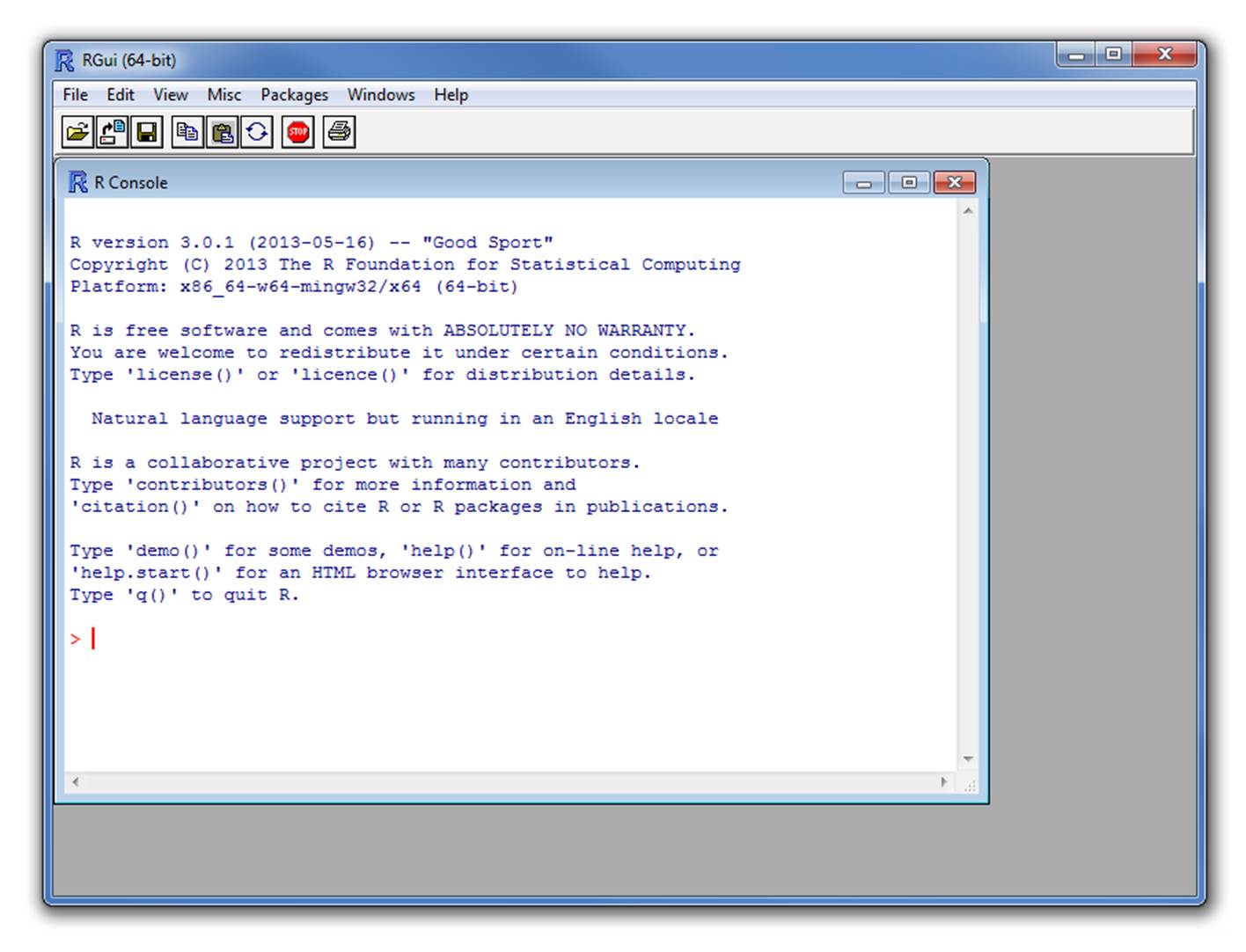
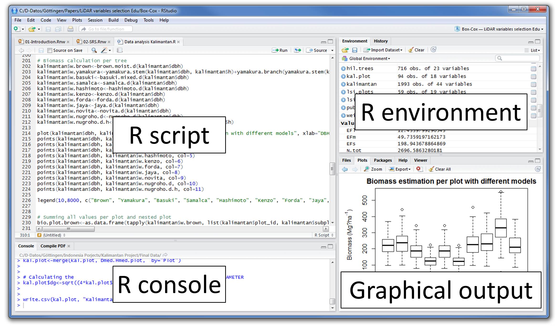
2 Rstudio

Integrated development environment (IDE) for R. Includes:

A console
Syntax highlighting editor supporting direct code execution
Tools for tracing, history, debugging, and workspace management

2.1

3 Elements of the R language

In R everything that exists is an object and objects can be roughly classified into objects that contain data and objects that perform tasks, better known as functions:

flowchart LR
    classDef largeText font-size:18px, padding:15px;

    R(Objects in R) --> D(Data objects)
    D --> D1(1 dimension)
    D --> D2(2 dimensions)
    D --> DN(N dimensions)
    R --> F(Functions)
    
    D1 --> V(Vector)
    D1 --> L(List)
    D2 --> M(Matrix)
    D2 --> DF(Data Frame)
    DN --> AR(Array)

    F --> BF(Integraded functions)
    BF --> BA(Basic functions)
    BF --> OP(Operators)
    F --> PF(Packages)
    F --> UF(User defined functions)

    class R,D,D1,D2,F largeText;

    style R fill:#28192F66, stroke:#000, stroke-width:2px, color:#FFF, width:140px
    style D fill:#40498E66, stroke:#000, stroke-width:2px, color:#FFF, width:180px
    style D1 fill:#348AA666, stroke:#000, stroke-width:2px, color:#FFF, width:140px
    style D2 fill:#348AA666, stroke:#000, stroke-width:2px, color:#FFF, width:140px
    style DN fill:#348AA666, stroke:#000, stroke-width:2px, color:#FFF, width:140px
    style F fill:#357BA266, stroke:#000, stroke-width:2px, color:#FFF, width:120px
    style DF fill:#49C1AD66, stroke:#000, stroke-width:2px, color:#000
    style AR fill:#49C1AD66, stroke:#000, stroke-width:2px, color:#000
    style V fill:#49C1AD66, stroke:#000, stroke-width:2px, color:#000
    style M fill:#49C1AD66, stroke:#000, stroke-width:2px, color:#000
    style L fill:#49C1AD66, stroke:#000, stroke-width:2px, color:#000
    style BF fill:#A0DFB966, stroke:#000, stroke-width:2px, color:#000
    style BA fill:#DEF5E566, stroke:#000, stroke-width:2px, color:#000
    style OP fill:#DEF5E566, stroke:#000, stroke-width:2px, color:#000    
    style PF fill:#A0DFB966, stroke:#000, stroke-width:2px, color:#000000
    style UF fill:#A0DFB966, stroke:#000, stroke-width:2px, color:#000

To feel comfortable programming in R it is necessary to know at all times what kind of objects we are working with. The class() and str() functions allow us to evaluate the structure of objects. We will be using them repeatedly in this tutorial.

3.1 Objects containing data

The basic data structure in R is the vector. With this all other object classes are built. To understand classes it is useful to think about the number of dimensions (1, 2 or more) and types of data they can contain: homogeneous (a single element type) or heterogeneous (or multiple element types).

flowchart LR
    classDef largeText font-size:18px, padding:15px;

    D(Data objects) --> D1(1 dimension)
    D --> D2(2 dimensions)
    D1 --> V(Vector)
    D1 --> L(List)
    D2 --> M(Matrix)
    D2 -->  DF(Data Frame)

    style D fill:#40498E66, stroke:#000, stroke-width:2px, color:#FFF, width:180px
    style D1 fill:#348AA666, stroke:#000, stroke-width:2px, color:#FFF, width:140px
    style D2 fill:#348AA666, stroke:#000, stroke-width:2px, color:#FFF, width:140px
    style DF fill:#49C1AD66, stroke:#000, stroke-width:2px, color:#000
    style V fill:#49C1AD66, stroke:#000, stroke-width:2px, color:#000
    style M fill:#49C1AD66, stroke:#000, stroke-width:2px, color:#000
    style L fill:#49C1AD66, stroke:#000, stroke-width:2px, color:#000

	Homogeneous	Heterogeneous
1d	Atomic vector	List
2d	Matrix	Data frame
nd	Array

3.1.1 1 dimension objects

There are two basic types of vectors: atomic vectors and lists.

They have three common properties:

Type, typeof() (class/mode).
Length, length() (number of elements)
Attributes, attributes() (metadata)

They differ in the types of their elements: all elements of an atomic vector must be of the same type, while the elements of a list can have different types.

3.1.1.1 Atomic vectors

Types of atomic vectors:

Logical (Boolean)
Integer
Numeric (double)
Characters
Factors

Vectors are constructed with the c() function, they can be numeric:

Code

x <- 1
x1 <- c(1)

all.equal(x, x1)

[1] TRUE

Code

class(x)

[1] "numeric"

Characters:

Code

y <- "something"

class(y)

[1] "character"

Logical:

Code

z <- TRUE

class(z)

[1] "logical"

Or factor:

Code

q <- factor(1)

class(q)

[1] "factor"

Therefore, the individual numbers or strings are actually vectors of length one:

Code

class(1)

[1] "numeric"

Code

class("a")

[1] "character"

Vectors can only contain elements of the same type. Different types of elements will be forced to the most flexible type:

Code

x <- c(1, 2, "a")

x

[1] "1" "2" "a"

Code

class(x)

[1] "character"

Missing values are specified with NA, which is a logical vector of length 1. NA will always be interpreted to the correct type if used inside c():

Code

v <- c(10, 11, NA)

class(v)

[1] "numeric"

Code

v <- c("a", "b", NA)

class(v)

[1] "character"

3.1.1.2 Factors

Vectors with factors are very similar to character vectors. However, a factor can only contain predefined values, known as levels. Attributes are used to define the levels of the factor.

Factors are built on integer vectors using two attributes:

“factor” class: makes them behave differently from normal character vectors.
levels: defines the set of allowed values

Code

x <- factor(c("a", "b", "b", "a"))
x

[1] a b b a
Levels: a b

Code

levels(x)

[1] "a" "b"

Code

str(x)

 Factor w/ 2 levels "a","b": 1 2 2 1

The factors look like character vectors, but are actually integers:

Code

x <- factor(c("a", "b", "b", "a"))

c(x)

[1] a b b a
Levels: a b

3.1.1.3 Lists

Can contain objects of different classes and sizes. Lists are constructed with list():

Code

l <- list("a", 1, FALSE)

l

[[1]]
[1] "a"

[[2]]
[1] 1

[[3]]
[1] FALSE

Code

class(l)

[1] "list"

Code

str(l)

List of 3
 $ : chr "a"
 $ : num 1
 $ : logi FALSE

In fact, they can be seen as drawers where you can put any other type of object:

Code

l <- list(c("a", "b"), 
          c(1, 2, 3, 4), 
          c(FALSE, TRUE, FALSE))

l

[[1]]
[1] "a" "b"

[[2]]
[1] 1 2 3 4

[[3]]
[1] FALSE  TRUE FALSE

Code

str(l)

List of 3
 $ : chr [1:2] "a" "b"
 $ : num [1:4] 1 2 3 4
 $ : logi [1:3] FALSE TRUE FALSE

3.1.2 2-dimensional objects

3.1.2.1 Matrices

All elements are of the same type:

Code

m <- matrix(c("a", "b", "c", "d", "e", "f"), nrow = 2)

dim(m)

[1] 2 3

Code

     [,1] [,2] [,3]
[1,] "a"  "c"  "e" 
[2,] "b"  "d"  "f"

Code

class(m)

[1] "matrix" "array"

Code

m <- matrix(c("a", "b", "c", "d", "e", 1), nrow = 2)
m

     [,1] [,2] [,3]
[1,] "a"  "c"  "e" 
[2,] "b"  "d"  "1"

3.1.2.2 Data Frames

Special case of lists. It can contain elements of different types:

Code

m <-
  data.frame(
    ID = c("a", "b", "c", "d", "e"),
    size = c(1, 2, 3, 4, 5),
    observed = c(FALSE, TRUE, FALSE, FALSE, FALSE)
  )

dim(m)

[1] 5 3

Code

ID	size	observed
a	1	FALSE
b	2	TRUE
c	3	FALSE
d	4	FALSE
e	5	FALSE

Code

class(m)

[1] "data.frame"

Code

is.data.frame(m)

[1] TRUE

Code

is.list(m)

[1] TRUE

Code

str(m)

'data.frame':   5 obs. of  3 variables:
 $ ID      : chr  "a" "b" "c" "d" ...
 $ size    : num  1 2 3 4 5
 $ observed: logi  FALSE TRUE FALSE FALSE FALSE

But the vectors must have the same length:

Code

m <-
  data.frame(
    ID = c("a", "b", "c", "d", "e"),
    size = c(1, 2, 3, 4, 5, 6),
    observed = c(FALSE, TRUE, FALSE, FALSE, FALSE)
  )

Error in data.frame(ID = c("a", "b", "c", "d", "e"), size = c(1, 2, 3, : arguments imply differing number of rows: 5, 6

3.2 Exercise 1

Create a numeric vector with 8 elements containing positive and negative numbers.
Create a character vector with the names of the provinces of Costa Rica.
Add to the above point vector an NA
Create a numeric matrix with 3 columns and 3 rows
Create a character matrix with 4 columns and 3 rows
What class of object is ‘iris’ and what are its dimensions (hint: iris is an object available by default in your environment)?
Create a data frame with a numeric column, a character column and a factor column.

3.3 Functions: objects that perform tasks

All functions are created with the function() function and follow the same structure:

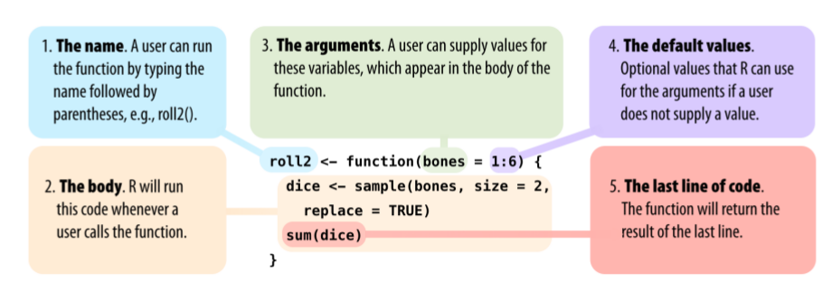
* Modified from Grolemund 2014

3.3.1 Integrated functions

3.3.1.1 Basic functions

R comes with many functions that you can use to do sophisticated tasks:

Code

# built in functions
bi <- builtins(internal = FALSE)

length(bi)

[1] 1406

Some functions come by default with R basic. New functions can be loaded as part of additional packages or even created by the user.

flowchart LR
    classDef largeText font-size:18px, padding:15px;

    F(Functions) --> BF(Integraded functions)
    BF --> OP(Operators)
    BF --> BA(Basic functions)
    F --> PF(Packages)
    F --> UF(User defined functions)

    class R,D,D1,D2,F largeText;

    style F fill:#357BA266, stroke:#000, stroke-width:2px, color:#FFF, width:120px
    style BF fill:#A0DFB966, stroke:#000, stroke-width:2px, color:#000
    style BA fill:#DEF5E566, stroke:#000, stroke-width:2px, color:#000
    style OP fill:#DEF5E566, stroke:#000, stroke-width:2px, color:#000    
    style PF fill:#A0DFB966, stroke:#000, stroke-width:2px, color:#000000
    style UF fill:#A0DFB966, stroke:#000, stroke-width:2px, color:#000

3.3.1.2 Operators

Operators are functions:

Code

1 + 1

[1] 2

Code

'+'(1, 1)

[1] 2

Code

2 * 3

[1] 6

Code

'*'(2, 3)

[1] 6

3.3.1.2.1 Most used operators

Arithmetic operators:

Operator	Description
+	sum
-	subtraction
*	multiplication
/	division
^ or **	exponential

Code

1 - 2

[1] -1

Code

1 + 2

[1] 3

Code

2 ^ 2

[1] 4

Code

2 ** 2

[1] 4

Code

2:3 %in% 2:4

[1] TRUE TRUE

Logical operators:

Operator	Description
<	lower than
<=	lower than or equal to
>	higher than
>=	higher than or equal to
==	exactly the same
!=	different than
!x	Is not x
x \| y	x O y
x & y	x Y y
x %in% y	correspondence

Code

1 < 2

[1] TRUE

Code

1 > 2

[1] FALSE

Code

1 <= 2

[1] TRUE

Code

1 == 2

[1] FALSE

Code

1 != 2

[1] TRUE

Code

1 > 2

[1] FALSE

Code

5 %in% 1:6

[1] TRUE

Code

5 %in% 1:4

[1] FALSE

3.3.2 Vectorization

Most functions are vectorized:

Code

1:6 * 1:6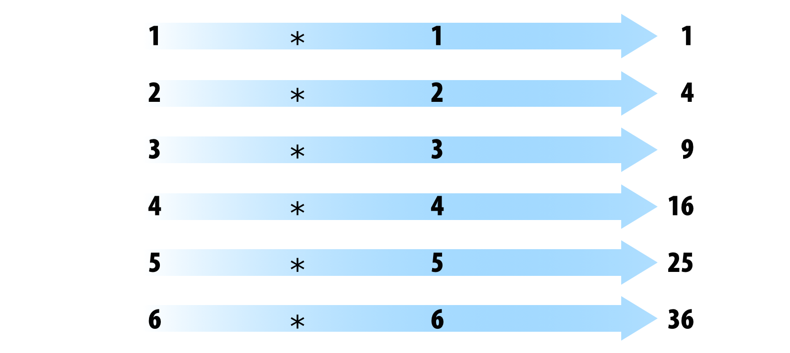

* Modified from Grolemund & Wickham 2017

[1]  1  4  9 16 25 36

Code

1:6 - 1:6

[1] 0 0 0 0 0 0

R recycles vectors of unequal length:

Code

1:6 * 1:5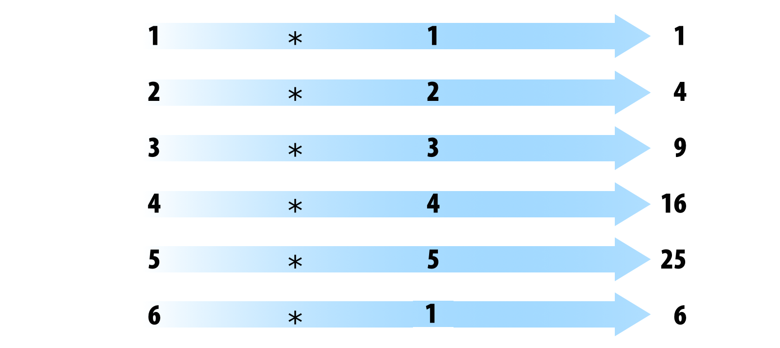

* Modified from Grolemund & Wickham 2017

3.3.3 Additional package functions

These are functions that are included in additional packages that can be installed and loaded into R. To be used the package must be installed and loaded, e.g. to use the corTest function of the “psych” package we must first install. The packages are installed from the CRAN (Comprehensive R Archive Network) server with the install.packages() function:

Code

install.packages("psych")

… and load the package:

Code

library(psych)

Once ‘psych’ is installed and loaded, we can call the corTest function:

Code

corTest(iris$Sepal.Length, iris$Sepal.Width)

Call:corTest(x = iris$Sepal.Length, y = iris$Sepal.Width)
Correlation matrix 
[1] -0.12
Sample Size 
[1] 150
These are the unadjusted probability values.
  The probability values  adjusted for multiple tests are in the p.adj object. 
[1] 0.15

 To see confidence intervals of the correlations, print with the short=FALSE option

The use of external packages is the most useful feature of R since it allows to make use of an almost infinite number of specialized functions in different tasks as well as in very diverse fields of science and industry.

We can explore the packages available for R at the CRAN website (click on the “packages” link).

3.4 Exercise 2

Search for a package you are interested in on CRAN
Install the package and load it
Run the example code of one of its functions

3.5 Object manipulation

3.6 Extracting subsets using indexing

Elements within objects can be called by indexing. To subset a vector simply call the position of the object using square brackets:

Code

x <- c("a", "b", "c", "d", "e", "a")

x[1]

[1] "a"

Code

x[2]

[1] "b"

Code

x[2:3]

[1] "b" "c"

Code

x[c(1,3)]

[1] "a" "c"

The elements can be removed in the same way:

Code

x[-1]

[1] "b" "c" "d" "e" "a"

Code

x[-c(1,3)]

[1] "b" "d" "e" "a"

The position of the indices can also be given by a conditional evaluation. For instance, this code selects the elements in x in which the value is “a”:

Code

x[x == "a"]

[1] "a" "a"

Notice that there are two steps in this process. First we create a logical vector in which TRUE means that the condition is met and FALSE that is not:

Code

is_a <- x == "a"

is_a

[1]  TRUE FALSE FALSE FALSE FALSE  TRUE

.. and then we use it to subset the data frame:

Code

x[is_a]

[1] "a" "a"

Conditional evaluations can also be used for numeric vectors (e.g. ‘>’, ‘==’) and to subset bidimensional objects based on columns or rows.

Matrices and data frames require 2 indices [row, column]:

Code

m <- matrix(c("a", "b", "c", "d", "e", "f"), nrow = 2)

m[1, ]

[1] "a" "c" "e"

Code

m[, 1]

[1] "a" "b"

Code

m[1, 1]

[1] "a"

Code

m[-1, ]

[1] "b" "d" "f"

Code

m[, -1]

     [,1] [,2]
[1,] "c"  "e" 
[2,] "d"  "f"

Code

m[-1, -1]

[1] "d" "f"

Code

df <- data.frame(
  provincia = c("San José", "Guanacaste", "Guanacaste"), 
  canton = c("Montes de Oca", "Nicoya", "Liberia"), 
    distrito = c("San Rafael", "Nosara", "Nacascolo")
  )

df

provincia	canton	distrito
San José	Montes de Oca	San Rafael
Guanacaste	Nicoya	Nosara
Guanacaste	Liberia	Nacascolo

Code

df[1, ]

provincia	canton	distrito
San José	Montes de Oca	San Rafael

Code

df[, 1]

[1] "San José"   "Guanacaste" "Guanacaste"

Code

df[1, 1]

[1] "San José"

Code

df[-1, ]

	provincia	canton	distrito
2	Guanacaste	Nicoya	Nosara
3	Guanacaste	Liberia	Nacascolo

Code

df[, -1]

canton	distrito
Montes de Oca	San Rafael
Nicoya	Nosara
Liberia	Nacascolo

Code

df[-1, -1]

	canton	distrito
2	Nicoya	Nosara
3	Liberia	Nacascolo

Data frames can also be subsetted using the name of the columns:

Code

df[,"provincia"]

[1] "San José"   "Guanacaste" "Guanacaste"

Code

df[,c("provincia", "canton")]

provincia	canton
San José	Montes de Oca
Guanacaste	Nicoya
Guanacaste	Liberia

Code

df$provincia

[1] "San José"   "Guanacaste" "Guanacaste"

Lists require 1 index between double square brackets [[index]]:

Code

l <- list(c("a", "b"),
          c(1, 2, 3),
          c(FALSE, TRUE, FALSE, FALSE))

l[[1]]

[1] "a" "b"

Code

l[[3]]

[1] FALSE  TRUE FALSE FALSE

Elements within lists can also be subsets in the same code string:

Code

l[[1]][1:2]

[1] "a" "b"

Code

l[[3]][2]

[1] TRUE

3.7 Explore objects

The following basic R functions (default) can help us to explore the structure of objects:

Code

str(df)

'data.frame':   3 obs. of  3 variables:
 $ provincia: chr  "San José" "Guanacaste" "Guanacaste"
 $ canton   : chr  "Montes de Oca" "Nicoya" "Liberia"
 $ distrito : chr  "San Rafael" "Nosara" "Nacascolo"

Code

names(df)

[1] "provincia" "canton"    "distrito"

Code

dim(df)

[1] 3 3

Code

nrow(df)

[1] 3

Code

ncol(df)

[1] 3

Code

head(df)

provincia	canton	distrito
San José	Montes de Oca	San Rafael
Guanacaste	Nicoya	Nosara
Guanacaste	Liberia	Nacascolo

Code

tail(df)

provincia	canton	distrito
San José	Montes de Oca	San Rafael
Guanacaste	Nicoya	Nosara
Guanacaste	Liberia	Nacascolo

Code

table(df$provincia)


Guanacaste   San José 
         2          1

Code

class(df)

[1] "data.frame"

Code

View(df)

3.8 Exercise 3

Use the example data iris to create a subset of data with only the observations of the species setosa.
Now create a subset of data containing the observations of both setosa and versicolor.
Also with iris create a subset of data with the observations for which iris$Sepal.length is greater than 6
How many observations have a sepal length greater than 6?

4 Style matters

Based on google’s R Style Guide

4.1 File names

File names must end in .R and, of course, be self-explanatory:

Good: graph_posterior_probability.R
Bad: graf.R

4.2 Object names

Variables and functions:

Lowercase
Use an underscore
In general, names for variables and verbs for functions.
Keep names concise and meaningful (not always easy).
Avoid using names of existing functions of variables

Code

- GOOD: day_one: day_1, mean_weight(),
  
- BAD: dayone, day1, first_day.of.month

4.3 Syntax

4.3.1 Spaces

Use spaces around operators and for arguments within a function.
Always put a space after a comma, and never before (as in normal English).
Place a space before the left parenthesis, except in a function call.

Code

  - GOOD: 
          a <- rnorm(n = 10, sd = 10, mean = 1)
          total <- sum(x[1, ])

  - BAD: 
         a<-rnorm(n=10,sd=10,mean=1) 
         total <- sum(x[,1])

4.3.1.1 Brackets

The opening key should never go on its own line.
The closing brace must always be on its own line.
You can omit braces when a block consists of only one statement

Code

  - GOOD:
              if (is.null(ylim)) {
              ylim <- c(0, 0.06)
            }
                      
            if (is.null(ylim))
              ylim <- c(0, 0.06)
          
  - BAD:
            
         if (is.null(ylim)) ylim <- c(0, 0.06)
                    
         if (is.null(ylim)) {ylim <- c(0, 0.06)} 

         if (is.null(ylim)) {
           ylim <- c(0, 0.06)
           }

4.3.1.2 Create objects

Use <-, instead of =

Code

  - GOOD:
         x <- 5 
          
  - BAD:
         x = 5

4.3.1.3 Suggestions to add comments

Comment your code
Entire commented lines should begin with # and a space.
Short comments can be placed after the code preceded by two spaces, #, and then a space.

Code

# Create histogram of frequency of campaigns by pct budget spent.
hist(df$pct.spent,
     breaks = "scott",  # method for choosing number of buckets
     main   = "Histogram: individuals per unit of time",
     xlab   = "Individual count",
     ylab   = "Frequency")

5 R Documentation

Most R resources are very well documented. So the first source of help you should turn to when writing R code is the R documentation itself. All packages are documented in the same standard way. Familiarizing yourself with the format can simplify things a lot.

5.1 Package documentation

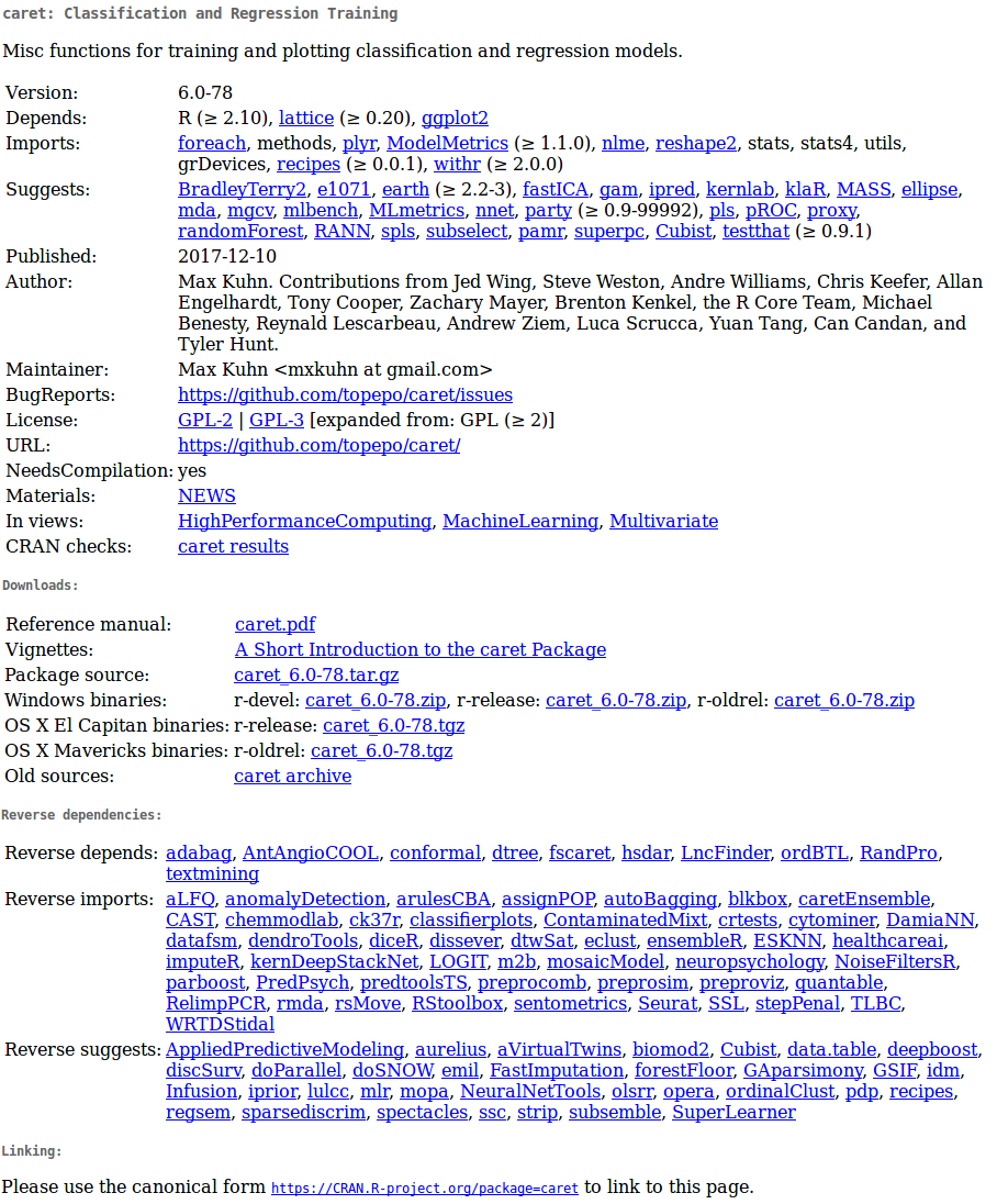
5.2 Reference manuals

Reference manuals are collections of documentation for all the functions of a package (only 1 per package):

5.3 Documentation of functions

All functions (default or loaded packages) must have documentation that follows a standard format:

Code

?mean

help("mean")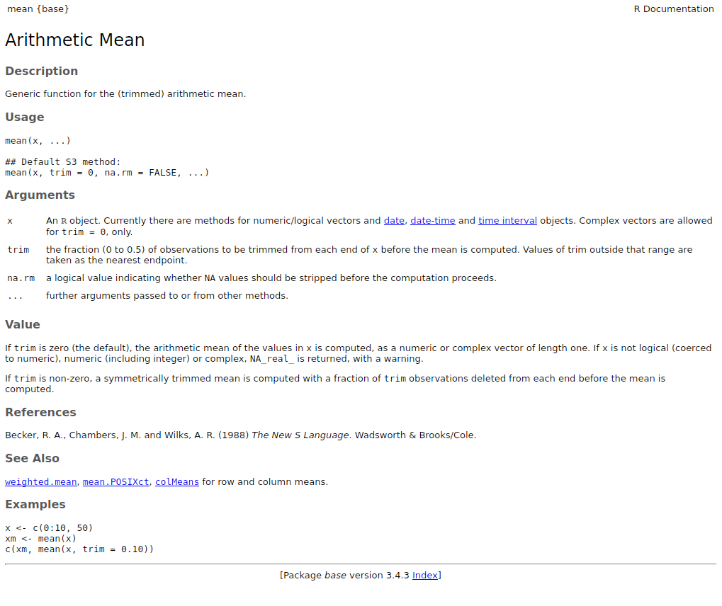

This documentation can also be displayed in Rstudio by pressing F1 when the cursor is on the function name.

If you do not remember the function name try apropos():

Code

apropos("mean")

 [1] ".colMeans"      ".rowMeans"      "circadian.mean" "circular.mean" 
 [5] "colMeans"       "geometric.mean" "harmonic.mean"  "kmeans"        
 [9] "mean"           "mean.Date"      "mean.default"   "mean.difftime" 
[13] "mean.POSIXct"   "mean.POSIXlt"   "rowMeans"       "weighted.mean" 
[17] "winsor.mean"    "winsor.means"

5.4 Vignettes (vignettes)

Vignettes are illustrative documents or case studies detailing the use of a package (optional, can be several per package).

Vignettes can be called directly from R:

Code

vgn <- browseVignettes()

Code

vignette()

También deberían aparecer en la página del paquete en CRAN.

5.5 Exercise 4

What does the cut() function do?
What is the breaks argument used for in cut()?
Run the first 4 lines of code from the examples provided in the cut() documentation.
How many bullets does the warbleR package have?

References

Advanced R, H Wickham
Google’s R Style Guide
Hands-On Programming with R (Grolemund, 2014)

Session info

R version 4.5.0 (2025-04-11)
Platform: x86_64-pc-linux-gnu
Running under: Ubuntu 22.04.5 LTS

Matrix products: default
BLAS:   /usr/lib/x86_64-linux-gnu/blas/libblas.so.3.10.0 
LAPACK: /usr/lib/x86_64-linux-gnu/lapack/liblapack.so.3.10.0  LAPACK version 3.10.0

locale:
 [1] LC_CTYPE=en_US.UTF-8       LC_NUMERIC=C              
 [3] LC_TIME=es_CR.UTF-8        LC_COLLATE=en_US.UTF-8    
 [5] LC_MONETARY=es_CR.UTF-8    LC_MESSAGES=en_US.UTF-8   
 [7] LC_PAPER=es_CR.UTF-8       LC_NAME=C                 
 [9] LC_ADDRESS=C               LC_TELEPHONE=C            
[11] LC_MEASUREMENT=es_CR.UTF-8 LC_IDENTIFICATION=C       

time zone: America/Costa_Rica
tzcode source: system (glibc)

attached base packages:
[1] stats     graphics  grDevices utils     datasets  methods   base     

other attached packages:
[1] psych_2.5.3

loaded via a namespace (and not attached):
 [1] vctrs_0.6.5        nlme_3.1-168       svglite_2.1.3      cli_3.6.5         
 [5] knitr_1.50         rlang_1.1.6        xfun_0.52          stringi_1.8.7     
 [9] jsonlite_2.0.0     glue_1.8.0         htmltools_0.5.8.1  scales_1.4.0      
[13] rmarkdown_2.29     grid_4.5.0         evaluate_1.0.3     kableExtra_1.4.0  
[17] fastmap_1.2.0      yaml_2.3.10        lifecycle_1.0.4    stringr_1.5.1     
[21] compiler_4.5.0     RColorBrewer_1.1-3 htmlwidgets_1.5.4  rstudioapi_0.17.1 
[25] lattice_0.22-7     systemfonts_1.2.3  farver_2.1.2       digest_0.6.37     
[29] viridisLite_0.4.2  R6_2.6.1           parallel_4.5.0     mnormt_2.1.1      
[33] magrittr_2.0.3     tools_4.5.0        xml2_1.3.8