<font size="7"><b>Introduction to warbleR</b></font> • warbleR

warbleR logo

The warbleR package is intended to facilitate the analysis of the structure of the animal acoustic signals in R. Users can enter their own data into a workflow that facilitates spectrographic visualization and measurement of acoustic parameters warbleR makes use of the fundamental sound analysis tools of the seewave package, and offers new tools for acoustic structure analysis. These tools are available for batch analysis of acoustic signals.

The main features of the package are:

The use of loops to apply tasks through acoustic signals referenced in a selection table
The production of image files with spectrograms that let users organize data and verify acoustic analyzes

The package offers functions for:

Browse and download recordings of Xeno-Canto
Explore, organize and manipulate multiple sound files
Detect signals automatically (in frequency and time)
Create spectrograms of complete recordings or individual signals
Run different measures of acoustic signal structure
Evaluate the performance of measurement methods
Catalog signals
Characterize different structural levels in acoustic signals
Statistical analysis of duet coordination
Consolidate databases and annotation tables

Most of the functions allow the parallelization of tasks, which distributes the tasks among several cores to improve computational efficiency. Tools to evaluate the performance of the analysis at each step are also available. All these tools are provided in a standardized workflow for the analysis of the signal structure, making them accessible to a wide range of users, including those without much knowledge of R. warbleR is a young package (officially published in 2017) currently in a maturation stage.

Selection tables

These objects are created with the selection_table() function. The function takes data frames containing selection data (name of the sound file, selection, start, end …), verifies if the information is consistent (see the function checksels() for details) and saves the ‘diagnostic’ metadata as an attribute. The selection tables are basically data frames in which the information contained has been corroborated so it can be read by other warbleR functions. The selection tables must contain (at least) the following columns:

sound files (sound.files)
selection (select)
start
end

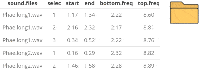
The sample data “lbh_selec_table” contains these columns:

data("lbh_selec_table")

lbh_selec_table

sound.files	channel	selec	start	end	bottom.freq	top.freq
Phae.long1.wav	1	1	1.1693549	1.3423884	2.220105	8.604378
Phae.long1.wav	1	2	2.1584085	2.3214565	2.169437	8.807053
Phae.long1.wav	1	3	0.3433366	0.5182553	2.218294	8.756604
Phae.long2.wav	1	1	0.1595983	0.2921692	2.316862	8.822316
Phae.long2.wav	1	2	1.4570585	1.5832087	2.284006	8.888027
Phae.long3.wav	1	1	0.6265520	0.7577715	3.006834	8.822316
Phae.long3.wav	1	2	1.9742132	2.1043921	2.776843	8.888027
Phae.long3.wav	1	3	0.1233643	0.2545812	2.316862	9.315153
Phae.long4.wav	1	1	1.5168116	1.6622365	2.513997	9.216586
Phae.long4.wav	1	2	2.9326920	3.0768784	2.579708	10.235116
Phae.long4.wav	1	3	0.1453977	0.2904966	2.579708	9.742279

… and can be converted to the selection_table format like this (after saving the corresponding sound files):

data(list = c("Phae.long1", "Phae.long2", "Phae.long3", "Phae.long4"))
writeWave(Phae.long1, file.path(tempdir(), "Phae.long1.wav"))
writeWave(Phae.long2, file.path(tempdir(), "Phae.long2.wav"))
writeWave(Phae.long3, file.path(tempdir(), "Phae.long3.wav"))
writeWave(Phae.long4, file.path(tempdir(), "Phae.long4.wav"))

# parametros globales
warbleR_options(wav.path = tempdir())

st <- selection_table(X = lbh_selec_table, pb = FALSE)

st

 [30mchecking selections (step 1 of 1): [39m

 [30mObject of class  [1m'selection_table' [22m [39m

 [90m* The output of the following call: [39m

 [90m [3mselection_table(X = lbh_selec_table, path = tempdir()) [23m [39m

 [90m [1m
Contains: [22m *  A selection table data frame with 11 rows and 7 columns: [39m

 [90m|sound.files    | channel| selec|  start|    end| bottom.freq| [39m

 [90m|:--------------|-------:|-----:|------:|------:|-----------:| [39m

 [90m|Phae.long1.wav |       1|     1| 1.1694| 1.3424|      2.2201| [39m

 [90m|Phae.long1.wav |       1|     2| 2.1584| 2.3215|      2.1694| [39m

 [90m|Phae.long1.wav |       1|     3| 0.3433| 0.5183|      2.2183| [39m

 [90m|Phae.long2.wav |       1|     1| 0.1596| 0.2922|      2.3169| [39m

 [90m|Phae.long2.wav |       1|     2| 1.4571| 1.5832|      2.2840| [39m

 [90m|Phae.long3.wav |       1|     1| 0.6266| 0.7578|      3.0068| [39m

 [90m... 1 more column(s) (top.freq) [39m

 [90m and 5 more row(s) [39m

 [90m
* A data frame (check.results) with 11 rows generated by check_sels() (as attribute) [39m

 [90mcreated by warbleR 1.1.30 [39m

Note that the path to the sound files has been provided. This is necessary in order to verify that the data provided conforms to the characteristics of the audio files.

Selection tables have their own class in R:

class(st)

[1] "selection_table" "data.frame"

Extended selection tables

When the extended = TRUE argument the function generates an object of the extended_selection_table class that also contains a list of ‘wave’ objects corresponding to each of the selections in the data. Therefore, the function transforms the selection table into self-contained objects since the original sound files are no longer needed to perform most of the acoustic analysis in warbleR. This can greatly facilitate the storage and exchange of (bio)acoustic data. In addition, it also speeds up analysis, since it is not necessary to read the sound files every time the data is analyzed.

Now, as mentioned earlier, you need the selection_table() function to create an extended selection table. You must also set the argument extended = TRUE (otherwise, the class would be a selection table). The following code converts the sample data into an extended selection table:

#  global parameters
warbleR_options(wav.path = tempdir())


ext_st <- selection_table(
  X = lbh_selec_table, 
  pb = FALSE,
  extended = TRUE
)

And that is. Now the acoustic data and the selection data (as well as the additional metadata) are all together in a single R object.

Handling extended selection tables

Several functions can be used to deal with objects of this class. You can test if the object belongs to the extended_selection_table:

is_extended_selection_table(ext_st)

[1] TRUE

You can subset the selection in the same way that any other data frame and it will still keep its attributes:

ext_st2 <- ext_st[1:2, ]

is_extended_selection_table(ext_st2)

[1] TRUE

There is also a generic version of print() for this class of objects:

## print
print(ext_st)

 [30mObject of class  [1m'extended_selection_table' [22m [39m

 [90m* The output of the following call: [39m

 [90m [3mselection_table(X = lbh_selec_table, extended = TRUE, pb = FALSE) [23m [39m

 [90m [1m
Contains: [22m 
*  A selection table data frame with 11 row(s) and 7 columns: [39m

 [90m|sound.files      | channel| selec| start|    end| bottom.freq| [39m

 [90m|:----------------|-------:|-----:|-----:|------:|-----------:| [39m

 [90m|Phae.long1.wav_1 |       1|     1|   0.1| 0.2730|      2.2201| [39m

 [90m|Phae.long1.wav_2 |       1|     1|   0.1| 0.2630|      2.1694| [39m

 [90m|Phae.long1.wav_3 |       1|     1|   0.1| 0.2749|      2.2183| [39m

 [90m|Phae.long2.wav_1 |       1|     1|   0.1| 0.2326|      2.3169| [39m

 [90m|Phae.long2.wav_2 |       1|     1|   0.1| 0.2262|      2.2840| [39m

 [90m|Phae.long3.wav_1 |       1|     1|   0.1| 0.2312|      3.0068| [39m

 [90m... 1 more column(s) (top.freq) [39m

 [90m and 5 more row(s) [39m

 [90m
* 11 wave object(s) (as attributes):  [39m

 [90mPhae.long1.wav_1, Phae.long1.wav_2, Phae.long1.wav_3, Phae.long2.wav_1, Phae.long2.wav_2, Phae.long3.wav_1 [39m

 [90m... and 5 more [39m

 [90m
* A data frame (check.results) with 11 rows generated by check_sels() (as attribute) [39m

 [90m
The selection table was created [3m [1m by element  [22m [23m(see 'class_extended_selection_table') [39m

 [90m* 1 sampling rate(s) (in kHz):  [1m22.5 [22m [39m

 [90m* 1 bit depth(s):  [1m16 [22m [39m

 [90m* Created by warbleR 1.1.30 [39m

… which is equivalent to:

ext_st

 [30mObject of class  [1m'extended_selection_table' [22m [39m

 [90m* The output of the following call: [39m

 [90m [3mselection_table(X = lbh_selec_table, extended = TRUE, pb = FALSE) [23m [39m

 [90m [1m
Contains: [22m 
*  A selection table data frame with 11 row(s) and 7 columns: [39m

 [90m|sound.files      | channel| selec| start|    end| bottom.freq| [39m

 [90m|:----------------|-------:|-----:|-----:|------:|-----------:| [39m

 [90m|Phae.long1.wav_1 |       1|     1|   0.1| 0.2730|      2.2201| [39m

 [90m|Phae.long1.wav_2 |       1|     1|   0.1| 0.2630|      2.1694| [39m

 [90m|Phae.long1.wav_3 |       1|     1|   0.1| 0.2749|      2.2183| [39m

 [90m|Phae.long2.wav_1 |       1|     1|   0.1| 0.2326|      2.3169| [39m

 [90m|Phae.long2.wav_2 |       1|     1|   0.1| 0.2262|      2.2840| [39m

 [90m|Phae.long3.wav_1 |       1|     1|   0.1| 0.2312|      3.0068| [39m

 [90m... 1 more column(s) (top.freq) [39m

 [90m and 5 more row(s) [39m

 [90m
* 11 wave object(s) (as attributes):  [39m

 [90mPhae.long1.wav_1, Phae.long1.wav_2, Phae.long1.wav_3, Phae.long2.wav_1, Phae.long2.wav_2, Phae.long3.wav_1 [39m

 [90m... and 5 more [39m

 [90m
* A data frame (check.results) with 11 rows generated by check_sels() (as attribute) [39m

 [90m
The selection table was created [3m [1m by element  [22m [23m(see 'class_extended_selection_table') [39m

 [90m* 1 sampling rate(s) (in kHz):  [1m22.5 [22m [39m

 [90m* 1 bit depth(s):  [1m16 [22m [39m

 [90m* Created by warbleR 1.1.30 [39m

You can also join them in rows. Here the original extended_selection_table is divided into 2 and bound again using rbind():

ext_st3 <- ext_st[1:5, ]

ext_st4 <- ext_st[6:11, ]

ext_st5 <- rbind(ext_st3, ext_st4)

# print
ext_st5

 [30mObject of class  [1m'extended_selection_table' [22m [39m

 [90m* The output of the following call: [39m

 [90m [3mrbind(deparse.level, ..1, ..2) [23m [39m

 [90m [1m
Contains: [22m 
*  A selection table data frame with 11 row(s) and 7 columns: [39m

 [90m|sound.files      | channel| selec| start|    end| bottom.freq| [39m

 [90m|:----------------|-------:|-----:|-----:|------:|-----------:| [39m

 [90m|Phae.long1.wav_1 |       1|     1|   0.1| 0.2730|      2.2201| [39m

 [90m|Phae.long1.wav_2 |       1|     1|   0.1| 0.2630|      2.1694| [39m

 [90m|Phae.long1.wav_3 |       1|     1|   0.1| 0.2749|      2.2183| [39m

 [90m|Phae.long2.wav_1 |       1|     1|   0.1| 0.2326|      2.3169| [39m

 [90m|Phae.long2.wav_2 |       1|     1|   0.1| 0.2262|      2.2840| [39m

 [90m|Phae.long3.wav_1 |       1|     1|   0.1| 0.2312|      3.0068| [39m

 [90m... 1 more column(s) (top.freq) [39m

 [90m and 5 more row(s) [39m

 [90m
* 11 wave object(s) (as attributes):  [39m

 [90mPhae.long1.wav_1, Phae.long1.wav_2, Phae.long1.wav_3, Phae.long2.wav_1, Phae.long2.wav_2, Phae.long3.wav_1 [39m

 [90m... and 5 more [39m

 [90m
* A data frame (check.results) with 11 rows generated by check_sels() (as attribute) [39m

 [90m
The selection table was created [3m [1m by element  [22m [23m(see 'class_extended_selection_table') [39m

 [90m* 1 sampling rate(s) (in kHz):  [1m22.5 [22m [39m

 [90m* 1 bit depth(s):  [1m16 [22m [39m

 [90m* Created by warbleR 1.1.30 [39m

# igual q el original
all.equal(ext_st, ext_st5)

[1] "Attributes: < Component \"call\": target, current do not match when deparsed >"

The ‘wave’ objects can be read individually using read_wave(), a wrapper for the readWave() function of tuneR, which can handle extended selection tables:

wv1 <- read_wave(X = ext_st, index = 3, from = 0, to = 0.37)

These are regular ‘wave’ objects:

class(wv1)

[1] "Wave"
attr(,"package")
[1] "tuneR"

wv1


Wave Object
    Number of Samples:      8325
    Duration (seconds):     0.37
    Samplingrate (Hertz):   22500
    Channels (Mono/Stereo): Mono
    PCM (integer format):   TRUE
    Bit (8/16/24/32/64):    16

spectro(wv1, wl = 150, grid = FALSE, scale = FALSE, ovlp = 90)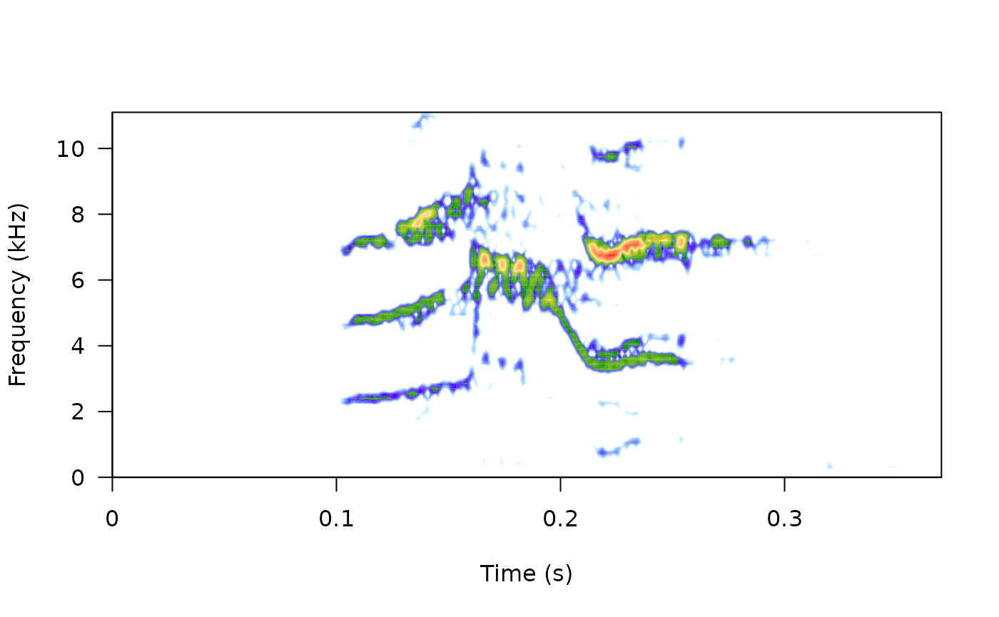

par(mfrow = c(3, 2), mar = rep(0, 4))

for (i in 1:6) {
  wv <- read_wave(X = ext_st, index = i, from = 0.05, to = 0.32)

  spectro(wv,
    wl = 150, grid = FALSE, scale = FALSE, axisX = FALSE,
    axisY = FALSE, ovlp = 90
  )
}

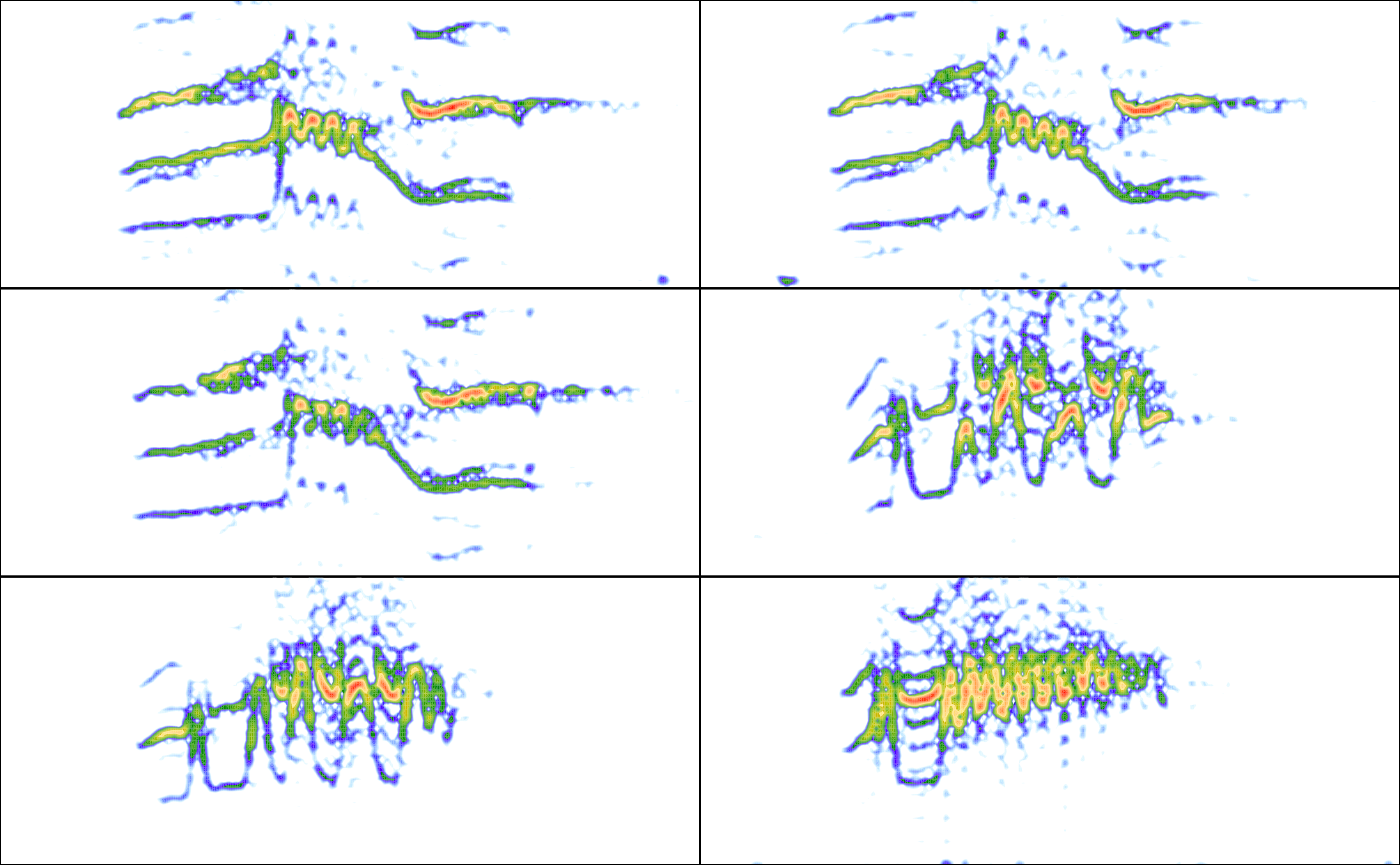
The read_wave() function requires the selection table, as well as the row index (i.e. the row number) to be able to read the ‘wave’ objects. It can also read a regular ‘wave’ file if the path is provided.

Note that other functions that modify data frames are likely to delete the attributes in which the ‘wave’ objects and metadata are stored. For example, the merge and the extended selection box will remove its attributes:

# create new data frame
Y <- data.frame(sound.files = ext_st$sound.files, site = "La Selva", lek = c(rep("SUR", 5), rep("CCL", 6)))

# combine
mrg_ext_st <- merge(ext_st, Y, by = "sound.files")

# check class
is_extended_selection_table(mrg_ext_st)

[1] FALSE

In this case, we can use the fix_extended_selection_table() function to transfer the attributes of the original extended selection table:

# fix est
mrg_ext_st <- fix_extended_selection_table(X = mrg_ext_st, Y = ext_st)

# check class
is_extended_selection_table(mrg_ext_st)

[1] TRUE

This works as long as some of the original sound files are retained and no other selections are added.

Analysis using extended selection tables

These objects can be used as input for most warbleR functions. Here are some examples of warbleR functions using extended_selection_table:

Spectral parameters

#  parametros espectrales
sp <- spectro_analysis(ext_st)

sp

Signal-to-noise ratio

snr <- sig2noise(ext_st, mar = 0.05)

snr

Dynamic time warping (DTW)

dtw.dist <- freq_DTW(ext_st, img = FALSE)

dtw.dist

Performance

The use of extended_selection_table objects can improve performance (in our case, measured as time). Here we use microbenchmark to compare the performance of sig2noise() and ggplot2 to plot the results. First, a selection table with 1000 selections is created simply by repeating the sample data frame several times and then is converted to an extended selection table:

# create long selection table
lng.selec.table <- do.call(rbind, replicate(10, lbh_selec_table,
  simplify = FALSE
))

# relabels selec
lng.selec.table$selec <- 1:nrow(lng.selec.table)

# create extended selection table
lng_ext_st <- selection_table(
  X = lng.selec.table, 
  pb = FALSE,
  extended = TRUE
  )


# load packages
library(microbenchmark)
library(ggplot2)

# check performance
mbmrk.snr <- microbenchmark(extended = sig2noise(lng_ext_st,
  mar = 0.05
), regular = sig2noise(lng.selec.table,
  mar = 0.05
), times = 50)

autoplot(mbmrk.snr) + ggtitle("sig2noise")

autodetec image example

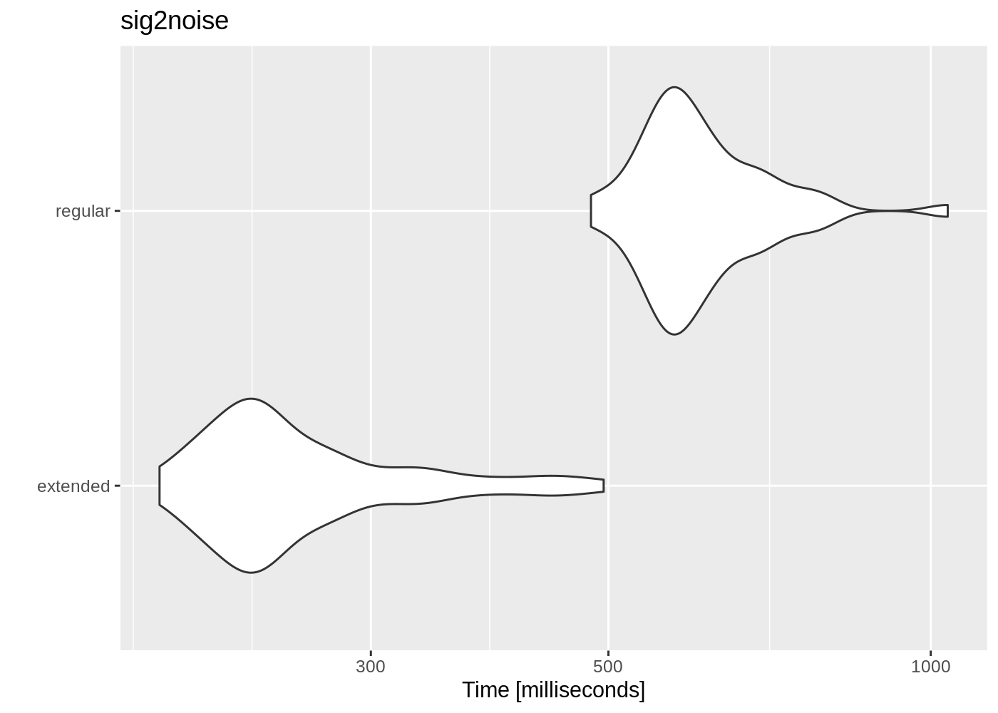
The function runs much faster in the extended selection tables. Performance gain is likely to improve when longer recordings and data sets are used (that is, to compensate for computing overhead).

This new object class allows to share complete data sets, including acoustic data. For example, the NatureSounds package contains an extended selection table with long-billed hermit hummingbirds vocalizations from 10 different song types:

data("Phae.long.est")

Phae.long.est

 [30mObject of class  [1m'extended_selection_table' [22m [39m

 [90m [1m
Contains: [22m 
*  A selection table data frame with 50 row(s) and 8 columns: [39m

 [90m|sound.files | selec| start|    end| bottom.freq| top.freq| [39m

 [90m|:-----------|-----:|-----:|------:|-----------:|--------:| [39m

 [90m|BR2-A1-1    |     1|   0.1| 0.2676|      1.6020|  10.9525| [39m

 [90m|BR2-A1-2    |     1|   0.1| 0.2652|      1.8914|  11.0250| [39m

 [90m|BR2-A1-3    |     1|   0.1| 0.2716|      1.7177|  11.0250| [39m

 [90m|BR2-A1-4    |     1|   0.1| 0.2701|      1.8335|  11.0250| [39m

 [90m|BR2-A1-5    |     1|   0.1| 0.2770|      2.1229|  11.0250| [39m

 [90m|CCE-I3-1    |     1|   0.1| 0.2490|      1.7551|  11.0250| [39m

 [90m... 2 more column(s) (lek, lek.song.type) [39m

 [90m and 44 more row(s) [39m

 [90m
* 50 wave object(s) (as attributes):  [39m

 [90mBR2-A1-1, BR2-A1-2, BR2-A1-3, BR2-A1-4, BR2-A1-5, CCE-I3-1 [39m

 [90m... and 44 more [39m

 [90m
* A data frame (check.results) with 50 rows generated by check_sels() (as attribute) [39m

 [90m
The selection table was created [3m [1m by element  [22m [23m(see 'class_extended_selection_table') [39m

 [90m* 1 sampling rate(s) (in kHz):  [1m22.05 [22m [39m

 [90m* 1 bit depth(s):  [1m8 [22m [39m

 [90m* Created by warbleR < 1.1.21 [39m

table(Phae.long.est$lek.song.type)


BR2-A1 CCE-I3 LOC-D1 SAT-F1 STR-A2 SUR-E1 SUR-K4 TR1-C2 TR1-C5 TR1-D4 
     5      5      5      5      5      5      5      5      5      5

The ability to compress large data sets and the ease of performing analyzes that require a single R object can simplify the exchange of data and the reproducibility of bioacoustic analyzes.

warbleR functions and the workflow of analysis in bioacoustics

Bioacoustic analyzes generally follow a specific processing sequence and analysis. This sequence can be represented schematically like this:

analysis workflow

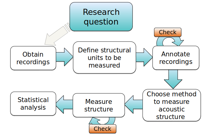
We can group warbleR functions according to the bioacoustic analysis stages.

Get and prepare recordings

The query_xc() function allows you to search and download sounds from the free access database Xeno-Canto. You can also convert .mp3 files to .wav, change the sampling rate of the files and correct corrupt files, among other functions.

Function	Description	Works on	Output
check_wavs	verify if sound files can be read	multiple wave files	data frame
consolidate	consolidate sound files in a single folder	multiple wave files	data frame and wave files
fix_wavs	fix waves that cannot be read in R	multiple wave files	wave files
mp32wav	convert multiple mp3 files to wav format	multiple mp3 files	wave files
query_xc	Search and download mp3 files from Xeno-Canto	Scientific names/data frame	mp3 files
resample_est	resample wave objects in ext. selection tables	extended selection tables	extended selection tables
remove_channels	remove channels in multiple wave files	multiple wave files	wave files
remove_silence	remove silences in multiple wave files	multiple wave files	wave files
duration_wavs	measures duration in multiple wave files	multiple wave files	data frame
info_wavs	extract recording parameters from multiple wave files	multiple wave files	data frame

Annotating sound

It is recommended to make annotations in other programs and then import them into R (for example in Raven and import them with the Rraven package). However, warbleR offers some functions to facilitate manual or automatic annotation of sound files, as well as the subsequent manipulation:

Function	Description	Works on	Output
auto_detec	automatic annotation of wave files	multiple wave files	data frame, images
freq_range	detect frequency range in selection tables	multiple wave files	data frame
tailor_sels	interactive tailoring of selections	selection tables	selection tables

Organize annotations

The annotations (or selection tables) can be manipulated and refined with a variety of functions. Selection tables can also be converted into the compact format extended selection tables:

Function	Description	Works on	Output
tailor_sels	interactive tailoring of selections	selection tables	selection tables
sort_colms	order columns in an intuitive way	selection tables	selection tables
cut_sels	save selections as individual wave files	selection tables	wave files
filter_sels	subset selection tables based on filtered image files	selection tables, ext. selection tables, images	selection tables, ext. selection tables
fix_extended_selection_table	add wave objects to extended selection tables	selection tables	extended selection tables
selection_table	create selection tables and extended selection tables	selection tables	selection tables, ext. selection tables
song_analysis	measures acoustic parameters at higher structural levels of organization	selection tables, ext. selection tables	data frame, selection tables

Measure acoustic signal structure

Most warbleR functions are dedicated to quantifying the structure of acoustic signals listed in selection tables using batch processing. For this, 4 main measurement methods are offered:

Spectrographic parameters
Cross correlation
Dynamic time warping (DTW)
Statistical descriptors of cepstral coefficients

Most functions gravitate around these methods, or variations of these methods:

Function	Description	Works on	Output
freq_range	detect frequency range in selection tables	multiple wave files	data frame
song_analysis	measures acoustic parameters at higher structural levels of organization	selection tables, ext. selection tables	data frame, selection tables
compare_methods	compare the performance of methods to measure acoustic structure	selection tables, ext. selection tables	images
freq_DTW	measures dynamic time warping (DTW) on dominant/fundamental frequency contours	selection tables, ext. selection tables	(di)similarity matrix, images
freq_ts	mesaures dominant/fundamental frequency contours	selection tables, ext. selection tables	data frame with frequency contours
inflections	measures number of inflections in frequency contours	data frame with frequency contours	data frame
mfcc_stats	measures statistical descriptors of Mel cepstral coefficients	selection tables, ext. selection tables	data frame
multi_DTW	measures dynamic time warping (DTW) on multiple contours	selection tables, ext. selection tables	(di)similarity matrix
sig2noise	measures signal-to-noise ratio	selection tables, ext. selection tables	selection tables, ext. selection tables
spectro_analysis	measures spectrographic parameters	selection tables, ext. selection tables	data frame
cross_correlation	measurec spectrographic cross-correlation	selection tables, ext. selection tables	(di)similarity matrix

Verify annotations

Functions are provided to detect inconsistencies in the selection tables or modify selection tables. The package also offers several functions to generate spectrograms showing the annotations, which can be organized by annotation categories. This allows you to verify if the annotations match the previously defined categories, which is particularly useful if the annotations were automatically generated.

Function	Description	Works on	Output
check_sels	double-check selection tables	selection tables	selection tables
overlapping_sels	finds (time) overlapping selections	selection tables, ext. selection tables	selection tables, ext. selection tables
catalog	creates spectrogram catalog	selection tables, ext. selection tables	images
catalog2pdf	convert catalogs to .pdf	images	images
spectrograms	create spectrogram images	selection tables, ext. selection tables	images
full_spectrograms	create spectrograms of whole sound files	multiple wave files, selection tables, ext. selection tables	images
full_spectrogram2pdf	convert full spectrograms to .pfg	images	images

Visually inspection of annotations and measurements

Function	Description	Works on	Output
snr_spectrograms	plots spectrograms highlighting areas where signal-to-noise ratio is measured	selection tables, ext. selection tables	images
spectrograms	create spectrogram images	selection tables, ext. selection tables	images
track_freq_contour	create spectrogram images including frequency contours	selection tables, ext. selection tables	images
plot_coordination	create schematic plots of coordinated signals	data frame	images
full_spectrograms	create spectrograms of whole sound files	multiple wave files, selection tables, ext. selection tables	images

Additional functions

Finally, warbleR offers functions to simplify the use of extended selection tables, organize large numbers of images with spectrograms and generate elaborated signal visualizations:

Function	Description	Works on	Output
is_extended_selection_table	check if object is extended selection tables	data frame	TRUE/FALSE
is_selection_table	check if object is selection tables	data frame	TRUE/FALSE
catalog2pdf	convert catalogs to .pdf	images	images
move_imgs	moves images among folders	images	images
map_xc	created maps from Xeno-Canto recordings	data frame	images
test_coordination	test statistical significance of vocal coordination	data frame	data frame
full_spectrogram2pdf	convert full spectrograms to .pfg	images	images
color_spectro	highlight signals with colors in a spectrogram	wave object	plot in R
freq_range_detec	detect frequency range in wave objetcs	wave object	data frame, plot in R
open_wd	open working directory
phylo_spectro	plots phylogenetic trees with spectrograms	selection tables	plot in R
read_wave	read wave files and wave objects	selection tables, ext. selection tables	wave object
sim_songs	simulate songs		wave object, wave file and selection table
tweak_spectro	creates mosaic plots with spectrograms with different display parameters	selection tables, ext. selection tables	images
warbleR_options	define global parameters for warbleR functions

References

Araya-Salas M, G Smith-Vidaurre & M Webster. 2017. Assessing the effect of sound file compression and background noise on measures of acoustic signal structure. Bioacoustics 4622, 1-17
Araya-Salas M, Smith-Vidaurre G (2017) warbleR: An R package to streamline analysis of animal acoustic signals. Methods Ecol Evol 8:184-191.

Session information

R version 4.3.2 (2023-10-31)
Platform: x86_64-pc-linux-gnu (64-bit)
Running under: Ubuntu 22.04.4 LTS

Matrix products: default
BLAS:   /usr/lib/x86_64-linux-gnu/openblas-pthread/libblas.so.3 
LAPACK: /usr/lib/x86_64-linux-gnu/openblas-pthread/libopenblasp-r0.3.20.so;  LAPACK version 3.10.0

locale:
 [1] LC_CTYPE=C.UTF-8       LC_NUMERIC=C           LC_TIME=C.UTF-8        LC_COLLATE=C.UTF-8    
 [5] LC_MONETARY=C.UTF-8    LC_MESSAGES=C.UTF-8    LC_PAPER=C.UTF-8       LC_NAME=C             
 [9] LC_ADDRESS=C           LC_TELEPHONE=C         LC_MEASUREMENT=C.UTF-8 LC_IDENTIFICATION=C   

time zone: UTC
tzcode source: system (glibc)

attached base packages:
[1] stats     graphics  grDevices utils     datasets  methods   base     

other attached packages:
[1] kableExtra_1.4.0   warbleR_1.1.30     NatureSounds_1.0.4 knitr_1.45         seewave_2.2.3     
[6] tuneR_1.4.6       

loaded via a namespace (and not attached):
 [1] sass_0.4.8        xml2_1.3.6        bitops_1.0-7      stringi_1.8.3     digest_0.6.34    
 [6] magrittr_2.0.3    evaluate_0.23     fastmap_1.1.1     jsonlite_1.8.8    brio_1.1.4       
[11] purrr_1.0.2       viridisLite_0.4.2 scales_1.3.0      pbapply_1.7-2     textshaping_0.3.7
[16] jquerylib_0.1.4   cli_3.6.2         rlang_1.1.3       fftw_1.0-8        munsell_0.5.0    
[21] cachem_1.0.8      yaml_2.3.8        tools_4.3.2       parallel_4.3.2    memoise_2.0.1    
[26] colorspace_2.1-0  vctrs_0.6.5       R6_2.5.1          proxy_0.4-27      lifecycle_1.0.4  
[31] dtw_1.23-1        stringr_1.5.1     fs_1.6.3          MASS_7.3-60       ragg_1.2.7       
[36] desc_1.4.3        pkgdown_2.0.7     bslib_0.6.1       glue_1.7.0        Rcpp_1.0.12      
[41] systemfonts_1.0.5 highr_0.10        xfun_0.42         rstudioapi_0.15.0 rjson_0.2.21     
[46] htmltools_0.5.7   rmarkdown_2.25    svglite_2.1.3     testthat_3.2.1    signal_1.8-0     
[51] compiler_4.3.2    RCurl_1.98-1.14

Introduction to warbleR

Marcelo Araya-Salas, PhD & Grace Smith-Vidaurre

2024-02-28

Selection tables

Extended selection tables

Handling extended selection tables

Analysis using extended selection tables

Spectral parameters

Signal-to-noise ratio

Dynamic time warping (DTW)

Performance

warbleR functions and the workflow of analysis in bioacoustics

Get and prepare recordings

Annotating sound

Organize annotations

Measure acoustic signal structure

Verify annotations

Visually inspection of annotations and measurements

Additional functions

References

Introduction to warbleR

Marcelo Araya-Salas, PhD & Grace Smith-Vidaurre

2024-02-28

Selection tables

Extended selection tables

Handling extended selection tables

Analysis using extended selection tables

Spectral parameters

Signal-to-noise ratio

Dynamic time warping (DTW)

Performance

Sharing acoustic data

warbleR functions and the workflow of analysis in bioacoustics

Get and prepare recordings

Annotating sound

Organize annotations

Measure acoustic signal structure

Verify annotations

Visually inspection of annotations and measurements

Additional functions

References