Case study

Objetive

Demonstrate how to articulate functions used during the course to obtain, explore and quantify acoustic data

1 Download Xeno-Canto data

The warbleR function query_xc() queries for avian vocalization recordings in the open-access online repository Xeno-Canto. It can return recordings metadata or download the associated sound files.

Get recording metadata for green hermits (Phaethornis guy):

Code

library(warbleR)

pg <- query_xc(qword = 'Phaethornis guy', download = FALSE)

Keep only song vocalizations of high quality:

Code

song_pg <- pg[grepl("song", ignore.case = TRUE, pg$Vocalization_type) & pg$Quality == "A", ]

# remove 1 site from Colombia to have a few samples per country
song_pg <- song_pg[song_pg$Locality != "Suaita, Santander", ]

Map locations using map_xc():

Code

map_xc(song_pg, leaflet.map = TRUE)

Once you feel fine with the subset of data you can go ahead and download the sound files and save the metadata as a .csv file:

Code

query_xc(X = song_pg, path = "./examples/p_guy", parallel = 3)

write.csv(song_pg, file = "./examples/p_guy/metadata_p_guy_XC.csv", row.names = FALSE)

2 Preparing sound files for analysis (optional)

Now convert all to .wav format (mp3_2_wav) and homogenizing sampling rate and bit depth (fix_wavs):

Code

mp3_2_wav(samp.rate = 22.05, path =  "./examples/p_guy")

fix_wavs(path =  "./examples/p_guy", samp.rate = 44.1, bit.depth = 16)

3 Annotating sound files in Raven

Now songs should be manually annotated and all the selection in the .txt files should be pooled together in a single spreadsheet.

4 Importing annotations into R

Once that is done we can read the spreadsheet with the package ‘readxl’ as follows:

Code

# install.packages("readxl") # install if needed

# load package
library(readxl)

# read data
annotations <- read_excel(path = "./examples/p_guy/annotations_p_guy.xlsx")

# check data
head(annotations)

selec	Channel	start	end	bottom.freq	top.freq	selec.file
1	1	0.7737	0.9939384	2.0962	7.7252	Phaethornis-guy-2022.Table.1.selections.txt
2	1	1.6837	1.9068363	2.0726	7.6074	Phaethornis-guy-2022.Table.1.selections.txt
3	1	10.1657	10.3917342	1.8371	8.0078	Phaethornis-guy-2022.Table.1.selections.txt
4	1	16.3237	16.5468363	2.0726	7.3248	Phaethornis-guy-2022.Table.1.selections.txt
5	1	1.6069	1.7517937	1.7193	8.7615	Phaethornis-guy-2022.Table.1.selections.txt
6	1	1.0129	1.1548958	1.7193	8.9264	Phaethornis-guy-2022.Table.1.selections.txt

Note that the column names should be: “start”, “end”, “bottom.freq”, “top.freq” and “sound.files”. In addition frequency columns (“bottom.freq” and “top.freq”) must be in kHz, not in Hz. We can check if the annotations are in the right format using warbleR’s check_sels():

Code

sound_file_path <- "./examples/p_guy/converted_sound_files/"

cs <- check_sels(annotations, path = sound_file_path)

all selections are OK

5 Measure acoustic structure

We can measured several parameters of acoustic structure with the warbleR function spectro_analysis():

Code

sp <- spectro_analysis(X = annotations, path = sound_file_path)

Then we summarize those parameters with a Principal Component Analysis (PCA):

Code

# run excluding sound file and selec columns
pca <- prcomp(sp[, -c(1, 2)])


# add first 2 PCs to sound file and selec columns
pca_data <- cbind(sp[, c(1, 2)], pca$x[, 1:2])

At this point should should get someting like this:

Code

head(pca_data)

sound.files	selec	PC1	PC2
Phaethornis-guy-227574.wav	1	-22.6069606	-13.127152
Phaethornis-guy-227574.wav	2	0.0586673	-17.321796
Phaethornis-guy-227574.wav	3	5.9795115	5.601346
Phaethornis-guy-227574.wav	4	-6.8159094	4.462788
Phaethornis-guy-238804.wav	5	11.2315003	6.895327
Phaethornis-guy-238804.wav	6	4.6828306	7.918963

‘PC1’ and ‘PC2’ are the 2 new dimensions that will be used to represent the acoustic space.

6 Adding metadata

Now we just need to add any metadata we considered important to try to explain acoustic similarities shown in the acoustic space scatterplot:

Code

# read XC metadata
song_pg <- read.csv("./examples/p_guy/metadata_p_guy_XC.csv")

# create a column with the file name in the metadata
song_pg$sound.files <- paste0(song_pg$Genus, "-", song_pg$Specific_epithet, "-", song_pg$Recording_ID, ".wav")

# and merge based on sound files and any metadata column we need
pca_data_md <- merge(pca_data, song_pg[, c("sound.files", "Country", "Latitude", "Longitude")])

7 Assessing geographic patterns of variation

We are ready to plot the acoustic space scatterplot. For this we will use the package ‘ggplot2’:

Code

# install.packages("ggplot2")
library(ggplot2)

# install.packages("viridis")
library(viridis)

Loading required package: viridisLite

Code

# plot
ggplot(data = pca_data_md, aes(x = PC1, y = PC2, color = Country, shape = Country)) +
  geom_point(size = 3) + 
  scale_color_viridis_d()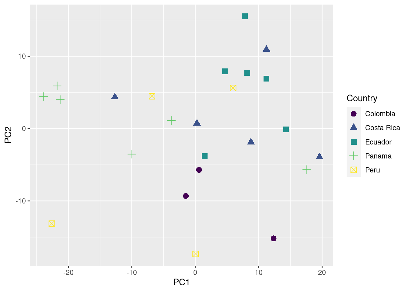

You can also add information about their geographic location (in this case longitude) to the plot as follows:

Code

# plot
ggplot(data = pca_data_md, aes(x = PC1, y = PC2, color = Longitude, shape = Country)) +
  geom_point(size = 3) +
  scale_color_viridis_c()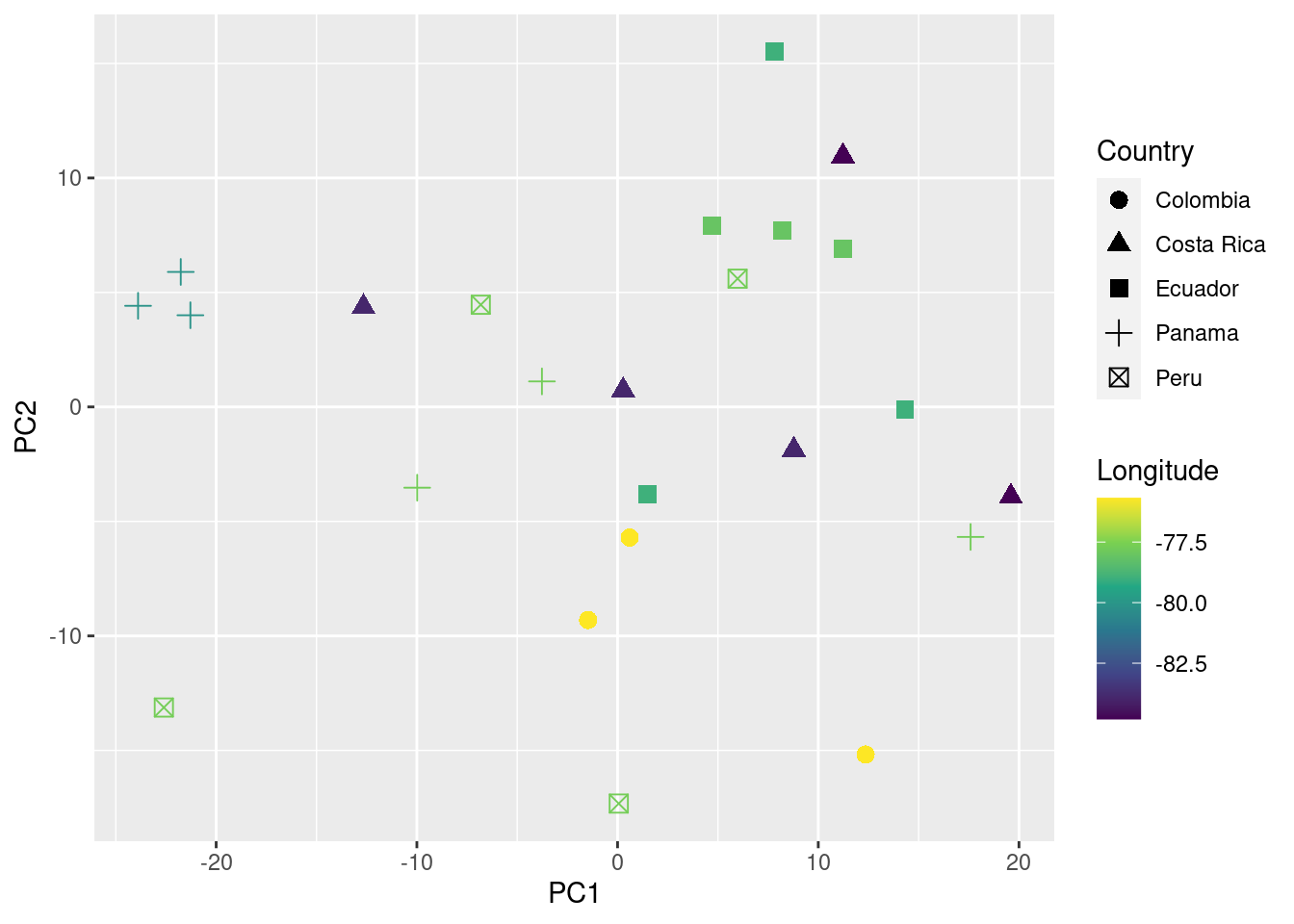

We can even test if geographic distance is associated to acoustic distance (i.e. if individuals geographically closer produce more similar songs) using a mantel test (mantel function from the package vegan):

Code

# create geographic and acoustic distance matrices
geo_dist <- dist(pca_data_md[, c("Latitude", "Longitude")])
acoust_dist <- dist(pca_data_md[, c("PC1", "PC2")])

# install.packages("vegan")
library(vegan)

# run test
mantel(geo_dist, acoust_dist)


Mantel statistic based on Pearson's product-moment correlation 

Call:
mantel(xdis = geo_dist, ydis = acoust_dist) 

Mantel statistic r: 0.02928 
      Significance: 0.235 

Upper quantiles of permutations (null model):
   90%    95%  97.5%    99% 
0.0669 0.1024 0.1397 0.1622 
Permutation: free
Number of permutations: 999

In this example no association between geographic and acoustic distance was detected (p value > 0.05).

Session information

R version 4.2.2 Patched (2022-11-10 r83330)
Platform: x86_64-pc-linux-gnu (64-bit)
Running under: Ubuntu 20.04.5 LTS

Matrix products: default
BLAS:   /usr/lib/x86_64-linux-gnu/blas/libblas.so.3.9.0
LAPACK: /usr/lib/x86_64-linux-gnu/lapack/liblapack.so.3.9.0

locale:
 [1] LC_CTYPE=es_ES.UTF-8       LC_NUMERIC=C              
 [3] LC_TIME=es_CR.UTF-8        LC_COLLATE=es_ES.UTF-8    
 [5] LC_MONETARY=es_CR.UTF-8    LC_MESSAGES=es_ES.UTF-8   
 [7] LC_PAPER=es_CR.UTF-8       LC_NAME=C                 
 [9] LC_ADDRESS=C               LC_TELEPHONE=C            
[11] LC_MEASUREMENT=es_CR.UTF-8 LC_IDENTIFICATION=C       

attached base packages:
[1] stats     graphics  grDevices utils     datasets  methods   base     

other attached packages:
 [1] vegan_2.6-4        lattice_0.20-45    permute_0.9-7      viridis_0.6.3     
 [5] viridisLite_0.4.2  ggplot2_3.4.2      readxl_1.4.1       warbleR_1.1.28    
 [9] NatureSounds_1.0.4 knitr_1.42         seewave_2.2.0      tuneR_1.4.4       

loaded via a namespace (and not attached):
 [1] Rcpp_1.0.10       fftw_1.0-7        digest_0.6.31     foreach_1.5.2    
 [5] utf8_1.2.3        R6_2.5.1          cellranger_1.1.0  signal_0.7-7     
 [9] evaluate_0.21     pillar_1.9.0      rlang_1.1.1       rstudioapi_0.14  
[13] Matrix_1.5-1      rmarkdown_2.21    splines_4.2.2     labeling_0.4.2   
[17] htmlwidgets_1.5.4 RCurl_1.98-1.12   munsell_0.5.0     proxy_0.4-27     
[21] compiler_4.2.2    xfun_0.39         pkgconfig_2.0.3   mgcv_1.8-41      
[25] htmltools_0.5.5   tidyselect_1.2.0  tibble_3.2.1      gridExtra_2.3    
[29] dtw_1.23-1        codetools_0.2-19  fansi_1.0.4       dplyr_1.1.0      
[33] withr_2.5.0       shinyBS_0.61.1    MASS_7.3-58.2     bitops_1.0-7     
[37] brio_1.1.3        grid_4.2.2        nlme_3.1-162      jsonlite_1.8.4   
[41] gtable_0.3.3      lifecycle_1.0.3   magrittr_2.0.3    scales_1.2.1     
[45] cli_3.6.1         pbapply_1.7-0     farver_2.1.1      leaflet_2.1.1    
[49] testthat_3.1.8    vctrs_0.6.2       generics_0.1.3    rjson_0.2.21     
[53] iterators_1.0.14  tools_4.2.2       glue_1.6.2        maps_3.4.1       
[57] crosstalk_1.2.0   parallel_4.2.2    fastmap_1.1.1     yaml_2.3.7       
[61] colorspace_2.1-0  cluster_2.1.4     soundgen_2.5.3