Introduction to warbleR

 

Objetive

• Provide and overview of the must relevant tools in the package warbleR

 

The warbleR package is intended to facilitate the analysis of the structure of animal acoustic signals in R. Users can enter their own data into a workflow that facilitates spectrographic visualization and measurement of acoustic parameters warbleR makes use of the fundamental sound analysis tools of the seewave package, and offers new tools for acoustic structure analysis. These tools are available for batch analysis of acoustic signals.

 

The main features of the package are:

• The use of loops to apply tasks through acoustic signals referenced in a selection table:

 

 

• The production of images files with spectrograms that let users organize data and verify acoustic analyzes:

 

 

The package offers functions for:

• Browse and download recordings of Xeno ‐ Canto
• Explore, organize and manipulate multiple sound files
• Detect signals automatically (in frequency and time)
• Create spectrograms of complete recordings or individual signals
• Run different measures of acoustic signal structure
• Evaluate the performance of measurement methods
• Catalog signals
• Characterize different structural levels in acoustic signals
• Statistical analysis of duet coordination
• Consolidate databases and annotation tables

Most functions allow the parallelization of tasks, which distributes the tasks among several cores to improve computational efficiency. Tools to evaluate the performance of the analysis at each step are also available. All these tools are provided in a standardized workflow for the analysis of the signal structure, making them accessible to a wide range of users, including those without much knowledge of R.

warbleR is a young package (officially published in 2017) currently in a maturation stage:

 

1 Selection tables

These objects are created with the selection_table() function. The function takes data frames containing selection data (name of the sound file, selection, start, end …), verifies if the information is consistent (see the function check_sels() for details) and saves the ‘diagnostic’ metadata as an attribute. The selection tables are basically data frames in which the information contained has been corroborated so it can be read by other warbleR functions. The selection tables must contain (at least) the following columns:

1. sound files (sound.files)
2. selection (select)
3. start
4. end

The sample data “lbh_selec_table” contains these columns:

Code

data("lbh_selec_table")

lbh_selec_table

sound.files	channel	selec	start	end	bottom.freq	top.freq
Phae.long1.wav	1	1	1.1693549	1.3423884	2.220105	8.604378
Phae.long1.wav	1	2	2.1584085	2.3214565	2.169437	8.807053
Phae.long1.wav	1	3	0.3433366	0.5182553	2.218294	8.756604
Phae.long2.wav	1	1	0.1595983	0.2921692	2.316862	8.822316
Phae.long2.wav	1	2	1.4570585	1.5832087	2.284006	8.888027
Phae.long3.wav	1	1	0.6265520	0.7577715	3.006834	8.822316
Phae.long3.wav	1	2	1.9742132	2.1043921	2.776843	8.888027
Phae.long3.wav	1	3	0.1233643	0.2545812	2.316862	9.315153
Phae.long4.wav	1	1	1.5168116	1.6622365	2.513997	9.216586
Phae.long4.wav	1	2	2.9326920	3.0768784	2.579708	10.235116
Phae.long4.wav	1	3	0.1453977	0.2904966	2.579708	9.742279

 

… and can be converted to the selection_table format like this:

Code

# global parameters
warbleR_options(wav.path = "./examples")

st <- selection_table(X = lbh_selec_table, pb = FALSE)

st

sound.files	channel	selec	start	end	bottom.freq	top.freq
Phae.long1.wav	1	1	1.1693549	1.3423884	2.220105	8.604378
Phae.long1.wav	1	2	2.1584085	2.3214565	2.169437	8.807053
Phae.long1.wav	1	3	0.3433366	0.5182553	2.218294	8.756604
Phae.long2.wav	1	1	0.1595983	0.2921692	2.316862	8.822316
Phae.long2.wav	1	2	1.4570585	1.5832087	2.284006	8.888027
Phae.long3.wav	1	1	0.6265520	0.7577715	3.006834	8.822316
Phae.long3.wav	1	2	1.9742132	2.1043921	2.776843	8.888027
Phae.long3.wav	1	3	0.1233643	0.2545812	2.316862	9.315153
Phae.long4.wav	1	1	1.5168116	1.6622365	2.513997	9.216586
Phae.long4.wav	1	2	2.9326920	3.0768784	2.579708	10.235116
Phae.long4.wav	1	3	0.1453977	0.2904966	2.579708	9.742279

Note that the path to the sound files has been provided. This is necessary in order to verify that the data provided conforms to the characteristics of the audio files.

Selection tables have their own class in R:

Code

class(st)

[1] "selection_table" "data.frame"     

 

1.1 Extended selection tables

When the extended = TRUE argument the function generates an object of the extended_selection_table class that also contains a list of ‘wave’ objects corresponding to each of the selections in the data. Therefore, the function transforms the selection table into self-contained objects since the original sound files are no longer needed to perform most of the acoustic analysis in warbleR. This can greatly facilitate the storage and exchange of (bio)acoustic data. In addition, it also speeds up analysis, since it is not necessary to read the sound files every time the data is analyzed.

Now, as mentioned earlier, you need the selection_table() function to create an extended selection table. You must also set the argument extended = TRUE (otherwise, the class would be a selection table). The following code converts the sample data into an extended selection table:

Code

#  global parameters
warbleR_options(wav.path = "./examples")

ext_st <- selection_table(X = lbh_selec_table, pb = FALSE, 
          extended = TRUE, confirm.extended = FALSE)

 

And that is. Now the acoustic data and the selection data (as well as the additional metadata) are all together in a single R object.

 

Exercise

 

• Run the example code in the selection_table() function documentation

• What do the arguments “mar”, “by.song” and “whole.recs” do?

 

1.2 Handling extended selection tables

Several functions can be used to deal with objects of this class. You can test if the object belongs to the extended_selection_table:

Code

is_extended_selection_table(ext_st)

[1] TRUE

 

You can subset the selection in the same way that any other data frame and it will still keep its attributes:

Code

ext_st2 <- ext_st[1:2, ]

is_extended_selection_table(ext_st2)

[1] TRUE

There is also a generic version of print() for this class of objects:

Code

## print
print(ext_st)

Object of class 'extended_selection_table'

* The output of the following call:

selection_table(X = lbh_selec_table, extended = TRUE, confirm.extended = FALSE,  pb = FALSE)

Contains: 
*  A selection table data frame with 11 row(s) and 7 columns:

|sound.files      | channel| selec| start|    end| bottom.freq|

|:----------------|-------:|-----:|-----:|------:|-----------:|

|Phae.long1.wav_1 |       1|     1|   0.1| 0.2730|      2.2201|

|Phae.long1.wav_2 |       1|     1|   0.1| 0.2630|      2.1694|

|Phae.long1.wav_3 |       1|     1|   0.1| 0.2749|      2.2183|

|Phae.long2.wav_1 |       1|     1|   0.1| 0.2326|      2.3169|

|Phae.long2.wav_2 |       1|     1|   0.1| 0.2262|      2.2840|

|Phae.long3.wav_1 |       1|     1|   0.1| 0.2312|      3.0068|

... 1 more column(s) (top.freq)

 and 5 more row(s)

* 11 wave object(s) (as attributes): 

Phae.long1.wav_1Phae.long1.wav_2Phae.long1.wav_3Phae.long2.wav_1Phae.long2.wav_2Phae.long3.wav_1

... and 5 more

* A data frame (check.results) generated by check_sels() (as attribute)

The selection table was created by element (see 'class_extended_selection_table')

* 1 sampling rate(s) (in kHz): 22.5

* 1 bit depth(s): 16

* Created by warbleR 1.1.28

… which is equivalent to:

Code

ext_st

Object of class 'extended_selection_table'

* The output of the following call:

selection_table(X = lbh_selec_table, extended = TRUE, confirm.extended = FALSE,  pb = FALSE)

Contains: 
*  A selection table data frame with 11 row(s) and 7 columns:

|sound.files      | channel| selec| start|    end| bottom.freq|

|:----------------|-------:|-----:|-----:|------:|-----------:|

|Phae.long1.wav_1 |       1|     1|   0.1| 0.2730|      2.2201|

|Phae.long1.wav_2 |       1|     1|   0.1| 0.2630|      2.1694|

|Phae.long1.wav_3 |       1|     1|   0.1| 0.2749|      2.2183|

|Phae.long2.wav_1 |       1|     1|   0.1| 0.2326|      2.3169|

|Phae.long2.wav_2 |       1|     1|   0.1| 0.2262|      2.2840|

|Phae.long3.wav_1 |       1|     1|   0.1| 0.2312|      3.0068|

... 1 more column(s) (top.freq)

 and 5 more row(s)

* 11 wave object(s) (as attributes): 

Phae.long1.wav_1Phae.long1.wav_2Phae.long1.wav_3Phae.long2.wav_1Phae.long2.wav_2Phae.long3.wav_1

... and 5 more

* A data frame (check.results) generated by check_sels() (as attribute)

The selection table was created by element (see 'class_extended_selection_table')

* 1 sampling rate(s) (in kHz): 22.5

* 1 bit depth(s): 16

* Created by warbleR 1.1.28

 

You can also join them in rows. Here the original extended_selection_table is divided into 2 and bound again using rbind():

Code

ext_st3 <- ext_st[1:5, ]

ext_st4 <- ext_st[6:11, ]

ext_st5 <- rbind(ext_st3, ext_st4)

#print
ext_st5

Object of class 'extended_selection_table'

* The output of the following call:

rbind(deparse.level, ..1, ..2)

Contains: 
*  A selection table data frame with 11 row(s) and 7 columns:

|sound.files      | channel| selec| start|    end| bottom.freq|

|:----------------|-------:|-----:|-----:|------:|-----------:|

|Phae.long1.wav_1 |       1|     1|   0.1| 0.2730|      2.2201|

|Phae.long1.wav_2 |       1|     1|   0.1| 0.2630|      2.1694|

|Phae.long1.wav_3 |       1|     1|   0.1| 0.2749|      2.2183|

|Phae.long2.wav_1 |       1|     1|   0.1| 0.2326|      2.3169|

|Phae.long2.wav_2 |       1|     1|   0.1| 0.2262|      2.2840|

|Phae.long3.wav_1 |       1|     1|   0.1| 0.2312|      3.0068|

... 1 more column(s) (top.freq)

 and 5 more row(s)

* 11 wave object(s) (as attributes): 

Phae.long1.wav_1Phae.long1.wav_2Phae.long1.wav_3Phae.long2.wav_1Phae.long2.wav_2Phae.long3.wav_1

... and 5 more

* A data frame (check.results) generated by check_sels() (as attribute)

The selection table was created by element (see 'class_extended_selection_table')

* 1 sampling rate(s) (in kHz): 22.5

* 1 bit depth(s): 16

* Created by warbleR 1.1.28

Code

# are they equal?
all.equal(ext_st, ext_st5)

[1] "Attributes: < Component \"call\": target, current do not match when deparsed >"

 

The ‘wave’ objects can be read individually using read_wave(), a wrapper for the readWave() function of tuneR, which can handle extended selection tables:

Code

wv1 <- read_wave(X = ext_st, index = 3, from = 0, to = 0.37)

 

These are regular ‘wave’ objects:

Code

class(wv1)

[1] "Wave"
attr(,"package")
[1] "tuneR"

Code

wv1

Wave Object
    Number of Samples:      8325
    Duration (seconds):     0.37
    Samplingrate (Hertz):   22500
    Channels (Mono/Stereo): Mono
    PCM (integer format):   TRUE
    Bit (8/16/24/32/64):    16 

Code

spectro(wv1, wl = 150, grid = FALSE, scale = FALSE, ovlp = 90)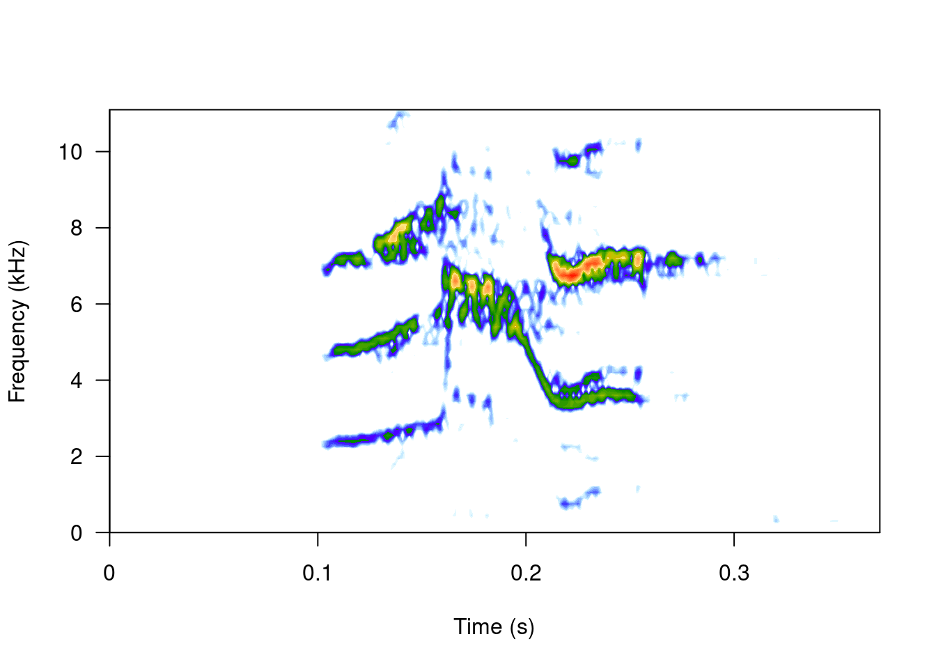

Code

par(mfrow = c(3, 2), mar = rep(0, 4))

for(i in 1:6){
  
  wv <- read_wave(X = ext_st, index = i, from = 0.05, to = 0.32)

  spectro(wv, wl = 150, grid = FALSE, scale = FALSE, axisX = FALSE,
          axisY = FALSE, ovlp = 90)

}

 

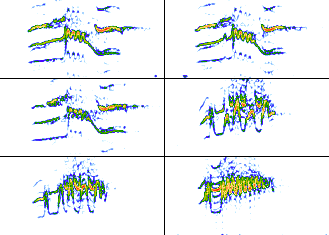
The read_wave() function requires the selection table, as well as the row index (i.e. the row number) to be able to read the ‘wave’ objects. It can also read a regular ‘wave’ file if the path is provided.

Note that other functions that modify data frames are likely to delete the attributes in which the ‘wave’ objects and metadata are stored. For example, the merge and the extended selection box will remove its attributes:

Code

# create new data base
Y <- data.frame(sound.files = ext_st$sound.files, site = "La Selva", lek = c(rep("SUR", 5), rep("CCL", 6)))

# combine
mrg_ext_st <- merge(ext_st, Y, by = "sound.files")

# check class
is_extended_selection_table(mrg_ext_st)

[1] FALSE

 

In this case, we can use the fix_extended_selection_table() function to transfer the attributes of the original extended selection table:

Code

# fix
mrg_ext_st <- fix_extended_selection_table(X = mrg_ext_st, Y = ext_st)

# check class
is_extended_selection_table(mrg_ext_st)

[1] TRUE

 

This works as long as some of the original sound files are retained and no other selections are added.

& nbsp;

1.3 Selection table size

The size of the extended selection box will depend on the number of selections, the sampling rate, the duration of the selection and the length of margins (i.e. additional time you want to keep on each side of the selection). In this example, a selection table with 1000 selections is created simply by repeating the sample data frame several times and then is converted to an extended selection table:

Code

lng.selec.table <- do.call(rbind, replicate(100, lbh_selec_table, 
                        simplify = FALSE))[1:1000,]

lng.selec.table$selec <- 1:nrow(lng.selec.table)

nrow(lng.selec.table)

lng_ext_st <- selection_table(X = lng.selec.table, pb = FALSE, 
                        extended = TRUE, confirm.extended = FALSE)

lng_ext_st

Object of class 'extended_selection_table'

* The output of the following call:

selection_table(X = lng.selec.table, extended = TRUE, confirm.extended = FALSE,  pb = FALSE)

Contains: 
*  A selection table data frame with 1000 row(s) and 7 columns:

|sound.files      | channel| selec| start|    end| bottom.freq|

|:----------------|-------:|-----:|-----:|------:|-----------:|

|Phae.long1.wav_1 |       1|     1|   0.1| 0.2730|      2.2201|

|Phae.long1.wav_2 |       1|     1|   0.1| 0.2630|      2.1694|

|Phae.long1.wav_3 |       1|     1|   0.1| 0.2749|      2.2183|

|Phae.long2.wav_4 |       1|     1|   0.1| 0.2326|      2.3169|

|Phae.long2.wav_5 |       1|     1|   0.1| 0.2262|      2.2840|

|Phae.long3.wav_6 |       1|     1|   0.1| 0.2312|      3.0068|

... 1 more column(s) (top.freq)

 and 994 more row(s)

* 1000 wave object(s) (as attributes): 

Phae.long1.wav_1Phae.long1.wav_2Phae.long1.wav_3Phae.long2.wav_4Phae.long2.wav_5Phae.long3.wav_6

... and 994 more

* A data frame (check.results) generated by check_sels() (as attribute)

The selection table was created by element (see 'class_extended_selection_table')

* 1 sampling rate(s) (in kHz): 22.5

* 1 bit depth(s): 16

* Created by warbleR 1.1.28

Code

format(object.size(lng_ext_st), units = "auto")

[1] "31.4 Mb"

 

As you can see, the object size is only ~ 31 MB. Then, as a guide, a selection box with 1000 selections similar to those of ‘lbh_selec_table’ (average duration of ~ 0.15 seconds) at a sampling rate of 22.5 kHz and the default margin (mar = 0.1) will generate an extended selection box ~ 31 MB or ~ 310 MB for a selection table of 10,000 rows.

 

1.4 Analysis using extended selection tables

These objects can be used as input for most warbleR functions. Here are some examples of warbleR functions using extended_selection_table:

1.4.1 Spectral parameters

Code

#  spectrographic parameters
sp <- spectro_analysis(ext_st)

sp

sound.files	selec	duration	meanfreq	sd	freq.median	freq.Q25	freq.Q75	freq.IQR	time.median	time.Q25	time.Q75	time.IQR	skew	kurt	sp.ent	time.ent	entropy	sfm	meandom	mindom	maxdom	dfrange	modindx	startdom	enddom	dfslope	meanpeakf
Phae.long1.wav_1	1	0.1730334	5.981221	1.399804	6.331716	5.296584	6.869521	1.572937	0.0798564	0.0532376	0.1197846	0.0665470	2.001382	7.025606	0.9434888	0.9493322	0.8956843	0.6518306	6.663993	5.251465	7.360840	2.109375	2.895833	7.316895	7.185059	-0.7619101	7.108806
Phae.long1.wav_2	1	0.1630480	5.997299	1.422930	6.212125	5.328746	6.880795	1.552049	0.0815333	0.0407667	0.1223000	0.0815333	1.918356	7.334323	0.9468217	0.9536154	0.9029038	0.6678647	6.830116	5.295410	8.283691	2.988281	2.661765	7.185059	7.229004	0.2695238	6.931635
Phae.long1.wav_3	1	0.1749187	6.018300	1.514853	6.424759	5.150246	6.979144	1.828898	0.0941949	0.0538256	0.1345641	0.0807385	2.496740	11.147728	0.9450838	0.9515916	0.8993339	0.6716602	6.773856	4.899902	8.371582	3.471680	3.240506	7.185059	7.185059	0.0000000	6.798757
Phae.long2.wav_1	1	0.1325709	6.398304	1.340412	6.595971	5.607323	7.380852	1.773529	0.0736543	0.0589235	0.1031160	0.0441926	1.568523	6.016392	0.9424661	0.9433998	0.8891223	0.6086184	6.341309	5.075684	7.404785	2.329102	2.830189	5.075684	6.657715	11.9334722	7.463147
Phae.long2.wav_2	1	0.1261502	6.308252	1.369242	6.596836	5.605837	7.207292	1.601455	0.0840889	0.0560593	0.0981037	0.0420444	2.470897	10.896039	0.9357725	0.9436684	0.8830589	0.6152336	6.411621	5.075684	7.580566	2.504883	2.087719	5.075684	7.580566	19.8563528	6.710171
Phae.long3.wav_1	1	0.1312195	6.605993	1.090498	6.665328	6.063201	7.336052	1.272851	0.0583111	0.0437333	0.1020444	0.0583111	1.770551	6.665163	0.9303558	0.9460672	0.8801790	0.5664857	6.481934	4.899902	7.009277	2.109375	1.520833	4.899902	6.965332	15.7402610	6.710171
Phae.long3.wav_2	1	0.1301789	6.639859	1.117356	6.674164	6.105325	7.427493	1.322168	0.0723210	0.0433926	0.1012494	0.0578568	1.545851	4.969900	0.9232849	0.9490351	0.8762298	0.5317422	6.244629	5.031738	6.701660	1.669922	1.368421	5.031738	6.613770	12.1527447	6.665879
Phae.long3.wav_3	1	0.1312170	6.580739	1.253000	6.646959	6.029463	7.394054	1.364591	0.0583111	0.0437333	0.1020444	0.0583111	1.802520	5.886959	0.9191879	0.9533815	0.8763367	0.5258369	6.231445	5.427246	6.833496	1.406250	1.656250	5.471191	6.657715	9.0424551	6.710171
Phae.long4.wav_1	1	0.1454249	6.219479	1.478869	6.233074	5.456261	7.305488	1.849227	0.0872533	0.0436267	0.1163378	0.0727111	1.274811	4.458109	0.9643357	0.9520564	0.9181020	0.7599268	6.270197	5.119629	7.844238	2.724609	2.709677	5.383301	6.262207	6.0437118	6.222951
Phae.long4.wav_2	1	0.1441864	6.462809	1.592876	6.338070	5.630777	7.572366	1.941589	0.0865067	0.0432533	0.1153422	0.0720889	1.695847	6.442755	0.9585943	0.9526078	0.9131645	0.7199148	6.294167	4.108887	8.151855	4.042969	2.478261	5.427246	4.108887	-9.1434347	6.222951
Phae.long4.wav_3	1	0.1450989	6.122156	1.541046	6.081716	5.178639	7.239860	2.061221	0.0870667	0.0435333	0.1160889	0.0725556	1.083042	4.194037	0.9642064	0.9536971	0.9195608	0.7332565	6.150346	4.943848	7.888184	2.944336	3.149254	5.339355	5.031738	-2.1200514	5.912903

 

1.4.2 Signal-to-noise ratio

Code

snr <- sig2noise(ext_st, mar = 0.05)

snr

sound.files	channel	selec	start	end	bottom.freq	top.freq	SNR
Phae.long1.wav_1	1	1	0.1	0.2730334	2.220105	8.604378	21.17229
Phae.long1.wav_2	1	1	0.1	0.2630480	2.169437	8.807053	20.36896
Phae.long1.wav_3	1	1	0.1	0.2749187	2.218294	8.756604	19.18211
Phae.long2.wav_1	1	1	0.1	0.2325709	2.316862	8.822316	23.27961
Phae.long2.wav_2	1	1	0.1	0.2261502	2.284006	8.888027	26.21774
Phae.long3.wav_1	1	1	0.1	0.2312195	3.006834	8.822316	25.34264
Phae.long3.wav_2	1	1	0.1	0.2301789	2.776843	8.888027	25.51099
Phae.long3.wav_3	1	1	0.1	0.2312170	2.316862	9.315153	24.68619
Phae.long4.wav_1	1	1	0.1	0.2454249	2.513997	9.216586	27.61899
Phae.long4.wav_2	1	1	0.1	0.2441864	2.579708	10.235116	28.87451
Phae.long4.wav_3	1	1	0.1	0.2450989	2.579708	9.742279	24.30149

 

1.4.3 Dynamic time warping (DTW)

Code

dtw.dist <- freq_DTW(ext_st, img = FALSE)

dtw.dist

Code

dtw.dist <- freq_DTW(ext_st, img = FALSE)

measuring dominant frequency contours (step 1 of 2): 

Measuring fundamental frequency:

calculating DTW distances (step 2 of 2, no progress bar):

Code

as.data.frame(dtw.dist)

	Phae.long1.wav_1-1	Phae.long1.wav_2-1	Phae.long1.wav_3-1	Phae.long2.wav_1-1	Phae.long2.wav_2-1	Phae.long3.wav_1-1	Phae.long3.wav_2-1	Phae.long3.wav_3-1	Phae.long4.wav_1-1	Phae.long4.wav_2-1	Phae.long4.wav_3-1
Phae.long1.wav_1-1	0.0000	8.6272	4.3390	16.6319	16.6161	13.8153	15.6860	15.5245	18.6621	20.8855	21.5606
Phae.long1.wav_2-1	8.6272	0.0000	6.9803	22.1235	29.1274	16.7363	22.3731	23.0249	15.8250	16.6372	19.4517
Phae.long1.wav_3-1	4.3390	6.9803	0.0000	18.2558	20.5344	15.2054	18.4506	16.4662	17.2609	19.1440	21.1586
Phae.long2.wav_1-1	16.6319	22.1235	18.2558	0.0000	12.1572	10.3686	11.2207	12.0419	12.4495	13.5389	15.3083
Phae.long2.wav_2-1	16.6161	29.1274	20.5344	12.1572	0.0000	6.7586	5.3403	8.6988	17.5231	20.5990	18.9194
Phae.long3.wav_1-1	13.8153	16.7363	15.2054	10.3686	6.7586	0.0000	3.6377	4.4201	13.2529	15.6284	15.6699
Phae.long3.wav_2-1	15.6860	22.3731	18.4506	11.2207	5.3403	3.6377	0.0000	3.6451	13.6515	15.9499	14.4185
Phae.long3.wav_3-1	15.5245	23.0249	16.4662	12.0419	8.6988	4.4201	3.6451	0.0000	11.0352	13.7203	12.3019
Phae.long4.wav_1-1	18.6621	15.8250	17.2609	12.4495	17.5231	13.2529	13.6515	11.0352	0.0000	5.3861	5.8845
Phae.long4.wav_2-1	20.8855	16.6372	19.1440	13.5389	20.5990	15.6284	15.9499	13.7203	5.3861	0.0000	6.2030
Phae.long4.wav_3-1	21.5606	19.4517	21.1586	15.3083	18.9194	15.6699	14.4185	12.3019	5.8845	6.2030	0.0000

 

1.5 Performance

The use of extended_selection_table objects can improve performance (in our case, measured as time). Here we use microbenchmark to compare the performance of sig2noise() and ggplot2 to plot the results:

Code

# load packages
library(microbenchmark)
library(ggplot2)

# take first 100 selections
mbmrk.snr <- microbenchmark(extended = sig2noise(lng_ext_st[1:100, ], 
      mar = 0.05), regular = sig2noise(lng.selec.table[1:100, ], 
                    mar = 0.05), times = 50)

autoplot(mbmrk.snr) + ggtitle("sig2noise")

Coordinate system already present. Adding new coordinate system, which will
replace the existing one.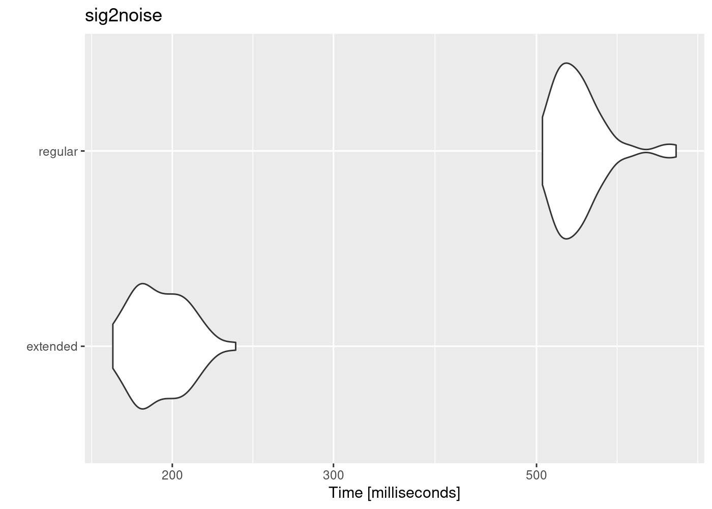

 

The function runs much faster in the extended selection tables. Performance gain is likely to improve when longer recordings and data sets are used (that is, to compensate for computer overload).

 

1.6 Create selections ‘by song’

The extended selection above were made by element. That is, each sound file within the object contains a single selection (that is, a 1: 1 correspondence between the selections and the ‘wave’ objects). However, extended selection tables can also be created using a higher hierarchical level with the argument by.song. In this case, “song” represents a higher level that contains one or more selections and that the user may want to keep together for a particular analysis (for example, the duration of the intervals). The by.song argument takes the name of the column of characters or factors with the IDs of the different” songs “within a sound file (note that the function assumes that a given song can only be found in only one sound file, so the selections with the same song ID, but from different sound files are taken as different ‘songs’).

To create a selection table by song, let’s add an artificial song column to our example data in which each of the sound files has 2 songs:

Code

# add column
lbh_selec_table$song <- c(1, 1, 2, 1, 2, 1, 1, 2, 1, 2, 2)

 

The data looks like this:

sound.files	channel	selec	start	end	bottom.freq	top.freq	song
Phae.long1.wav	1	1	1.1693549	1.3423884	2.220105	8.604378	1
Phae.long1.wav	1	2	2.1584085	2.3214565	2.169437	8.807053	1
Phae.long1.wav	1	3	0.3433366	0.5182553	2.218294	8.756604	2
Phae.long2.wav	1	1	0.1595983	0.2921692	2.316862	8.822316	1
Phae.long2.wav	1	2	1.4570585	1.5832087	2.284006	8.888027	2
Phae.long3.wav	1	1	0.6265520	0.7577715	3.006834	8.822316	1
Phae.long3.wav	1	2	1.9742132	2.1043921	2.776843	8.888027	1
Phae.long3.wav	1	3	0.1233643	0.2545812	2.316862	9.315153	2
Phae.long4.wav	1	1	1.5168116	1.6622365	2.513997	9.216586	1
Phae.long4.wav	1	2	2.9326920	3.0768784	2.579708	10.235116	2
Phae.long4.wav	1	3	0.1453977	0.2904966	2.579708	9.742279	2

 

Now we can create an extended selection table ‘by song’ using the column name ‘song’ as input for the argument by.song:

Code

bs_ext_st <- selection_table(X = lbh_selec_table, extended = TRUE,
                              confirm.extended = FALSE, by.song = "song")

checking selections (step 1 of 2):

saving wave objects into extended selection table (step 2 of 2):

In this case, we should only have 8 ‘wave’ objects instead of 11 as when the object was created ‘by selection’:

Code

# by element
length(attr(ext_st, "wave.objects"))

[1] 11

Code

# by song
length(attr(bs_ext_st, "wave.objects"))

[1] 8

Again, these objects can also be used in any analyzes:

Code

# signal to noise ratio
bs_snr <- sig2noise(bs_ext_st, mar = 0.05)

bs_snr

sound.files	channel	selec	start	end	bottom.freq	top.freq	song	SNR
Phae.long1.wav-song_1	1	1	0.100000	0.2730334	2.220105	8.604378	1	21.17229
Phae.long1.wav-song_1	1	2	1.089054	1.2521016	2.169437	8.807053	1	20.37064
Phae.long1.wav-song_2	1	1	0.100000	0.2749187	2.218294	8.756604	2	19.18211
Phae.long2.wav-song_1	1	1	0.100000	0.2325709	2.316862	8.822316	1	23.27961
Phae.long2.wav-song_2	1	1	0.100000	0.2261502	2.284006	8.888027	2	26.21774
Phae.long3.wav-song_1	1	1	0.100000	0.2312195	3.006834	8.822316	1	25.34264
Phae.long3.wav-song_1	1	2	1.447661	1.5778402	2.776843	8.888027	1	25.51089
Phae.long3.wav-song_2	1	1	0.100000	0.2312170	2.316862	9.315153	2	24.68619
Phae.long4.wav-song_1	1	1	0.100000	0.2454249	2.513997	9.216586	1	27.61899
Phae.long4.wav-song_2	1	1	2.887294	3.0314808	2.579708	10.235116	2	28.88520
Phae.long4.wav-song_2	1	2	0.100000	0.2450989	2.579708	9.742279	2	24.30149

 

Exercise

 

• Compare the size of an extended selection table created by element to that of one created by song using the sample data

 

1.7 Sharing acoustic data

This new object class allows to share complete data sets, including acoustic data. For example, the following code downloads a subset of the data used in Araya-Salas et al (2017) (can also be downloaded from here):

Code

URL <- "https://github.com/maRce10/OTS_BIR_2023/raw/master/data/extended.selection.table.araya-salas.et.al.2017.bioacoustics.100.sels.rds"

dat <- readRDS(gzcon(url(URL)))

nrow(dat)

format(object.size(dat), units = "auto")

[1] 100

[1] "10.1 Mb"

The total size of the 100 sound files from which these selections were taken adds up to 1.1 GB. The size of the extended selection table is only 10.1 MB.

This data is ready to be used:

Code

sp <- spectro_analysis(dat, bp = c(2, 10))

head(sp)

sound.files	selec	duration	meanfreq	sd	freq.median	freq.Q25	freq.Q75	freq.IQR	time.median	time.Q25	time.Q75	time.IQR	skew	kurt	sp.ent	time.ent	entropy	sfm	meandom	mindom	maxdom	dfrange	modindx	startdom	enddom	dfslope	meanpeakf
Pyrrhura rupicola Macaulay Library 132 .wav_2	1	0.1504762	4.662762	1.767083	4.279070	3.435216	5.647841	2.212625	0.0654244	0.0392547	0.1046791	0.0654244	2.619410	12.031225	0.9236435	0.9508231	0.8782216	0.5423756	3.753955	2.024121	6.847559	4.823437	5.375000	4.521973	2.024121	-16.599644	4.020775
0.CCE.1971.4.4.ITM70863A-23.wav_1	1	0.1655637	6.254850	1.648434	6.350453	5.601209	7.202417	1.601209	0.0827778	0.0382051	0.1209829	0.0827778	2.380005	10.144155	0.9397550	0.9410405	0.8843475	0.6327902	6.585970	3.574512	8.225684	4.651172	3.685185	8.225684	6.933691	-7.803594	6.096101
0.SAT.1989.6.2.ITM70866A-32.wav_5	1	0.1542514	6.093311	1.645878	5.844408	4.904376	7.393841	2.489465	0.0835469	0.0449868	0.1156803	0.0706935	1.970903	7.268969	0.9391274	0.9432334	0.8858163	0.6084129	6.234293	3.316113	8.139551	4.823437	3.214286	6.416894	3.316113	-20.102130	7.047292
23.CCE.2011.7.21.7.42.wav_6	1	0.1549551	5.415047	1.463110	5.167742	4.419355	6.425807	2.006452	0.0645692	0.0387415	0.1033107	0.0645692	2.107408	8.054270	0.9227024	0.9447503	0.8717234	0.5060075	5.028434	2.368652	7.795020	5.426367	2.158730	7.364356	2.368652	-32.239682	4.366662
Cyanoliseus patagonus Macaulay Library 79 .wav_5	1	0.1598866	3.153826	1.225681	2.569195	2.243941	3.651290	1.407350	0.0639546	0.0383728	0.0959320	0.0575592	4.547286	29.491407	0.8230714	0.9356593	0.7701144	0.1265239	2.590610	2.024121	4.435840	2.411719	3.071429	2.454785	2.282519	-1.077424	2.291336
0.HC1.2011.8.7.9.20.wav_4	1	0.1537989	6.029456	1.757841	6.416260	4.920325	7.183740	2.263415	0.0769048	0.0448611	0.1089484	0.0640873	4.161163	27.901632	0.9288549	0.9459573	0.8786571	0.6043575	6.254965	4.952637	8.570215	3.617578	4.071429	5.383301	4.952637	-2.800177	4.971966

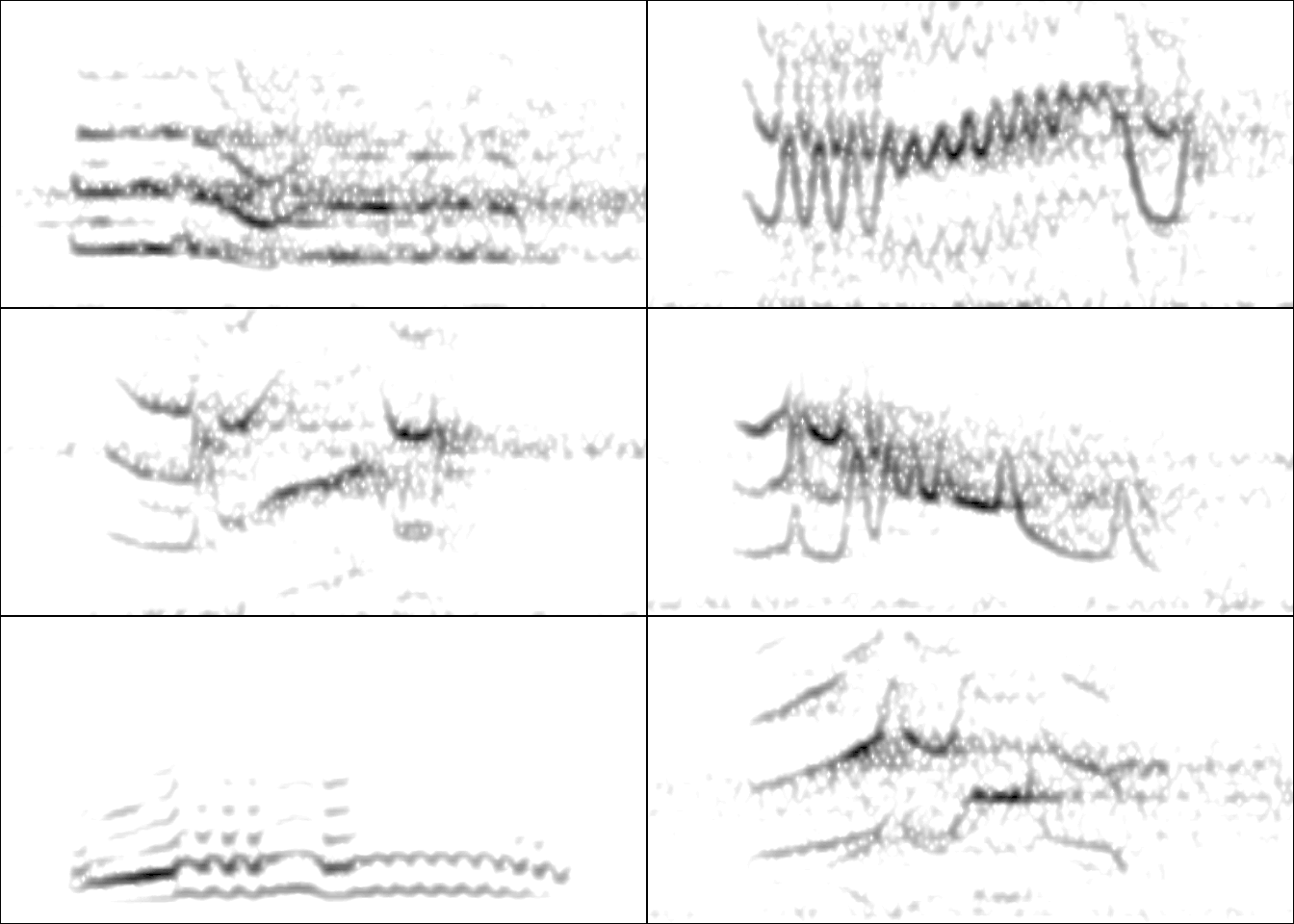
… and the spectrograms can be visualized as follows:

Code

par(mfrow = c(3, 2), mar = rep(0, 4))

for(i in 1:6){
  
  wv <- read_wave(X = dat, index = i, from = 0.17, to = 0.4)

  spectro(wv, wl = 250, grid = FALSE, scale = FALSE, axisX = FALSE,
          axisY = FALSE, ovlp = 90, flim = c(0, 12), 
          palette = reverse.gray.colors.1)
}

The NatureSounds package contains an extended selection table with long-billed hermit hummingbirds vocalizations from 10 different song types:

Code

data("Phae.long.est")

Phae.long.est

sound.files	selec	start	end	bottom.freq	top.freq	lek	lek.song.type
BR2-A1-1	1	0.1	0.2676122	1.601978	10.95248	BR2	BR2-A1
BR2-A1-2	1	0.1	0.2652138	1.891390	11.02500	BR2	BR2-A1
BR2-A1-3	1	0.1	0.2716211	1.717743	11.02500	BR2	BR2-A1
BR2-A1-4	1	0.1	0.2700891	1.833508	11.02500	BR2	BR2-A1
BR2-A1-5	1	0.1	0.2769735	2.122920	11.02500	BR2	BR2-A1
CCE-I3-1	1	0.1	0.2489883	1.755128	11.02500	CCE	CCE-I3
CCE-I3-2	1	0.1	0.2542084	1.621870	10.97237	CCE	CCE-I3
CCE-I3-3	1	0.1	0.2511759	1.710708	11.02500	CCE	CCE-I3
CCE-I3-4	1	0.1	0.2112061	1.932805	11.02500	CCE	CCE-I3
CCE-I3-5	1	0.1	0.2551176	1.533031	10.88353	CCE	CCE-I3
LOC-D1-1	1	0.1	0.2349864	1.204700	10.55520	LOC	LOC-D1
LOC-D1-2	1	0.1	0.2284810	1.387300	10.73780	LOC	LOC-D1
LOC-D1-3	1	0.1	0.2276679	1.387300	10.73780	LOC	LOC-D1
LOC-D1-4	1	0.1	0.2252284	1.533300	10.88380	LOC	LOC-D1
LOC-D1-5	1	0.1	0.2398654	2.336400	11.02500	LOC	LOC-D1
SAT-F1-1	1	0.1	0.2327233	1.577451	10.92795	SAT	SAT-F1
SAT-F1-2	1	0.1	0.2368484	1.755128	11.02500	SAT	SAT-F1
SAT-F1-3	1	0.1	0.2320470	1.804718	11.02500	SAT	SAT-F1
SAT-F1-4	1	0.1	0.2328000	1.767014	11.02500	SAT	SAT-F1
SAT-F1-5	1	0.1	0.2330560	1.842421	11.02500	SAT	SAT-F1
STR-A2-1	1	0.1	0.2229370	1.729311	11.02500	STR	STR-A2
STR-A2-2	1	0.1	0.2252280	1.653903	11.00440	STR	STR-A2
STR-A2-3	1	0.1	0.2236880	1.767014	11.02500	STR	STR-A2
STR-A2-4	1	0.1	0.2208320	1.767014	11.02500	STR	STR-A2
STR-A2-5	1	0.1	0.2280000	1.616200	10.96670	STR	STR-A2
SUR-E1-1	1	0.1	0.2398189	2.066063	11.02500	SUR	SUR-E1
SUR-E1-2	1	0.1	0.2385804	2.110482	11.02500	SUR	SUR-E1
SUR-E1-3	1	0.1	0.2383356	2.110482	11.02500	SUR	SUR-E1
SUR-E1-4	1	0.1	0.2408430	2.066063	11.02500	SUR	SUR-E1
SUR-E1-5	1	0.1	0.2358013	1.932805	11.02500	SUR	SUR-E1
SUR-K4-1	1	0.1	0.2357996	1.934900	11.02500	SUR	SUR-K4
SUR-K4-2	1	0.1	0.2317337	2.044400	11.02500	SUR	SUR-K4
SUR-K4-3	1	0.1	0.2276679	2.080900	11.02500	SUR	SUR-K4
SUR-K4-4	1	0.1	0.2284810	2.007900	11.02500	SUR	SUR-K4
SUR-K4-5	1	0.1	0.2382391	2.044400	11.02500	SUR	SUR-K4
TR1-C2-1	1	0.1	0.1926348	2.865609	11.02500	TR1	TR1-C2
TR1-C2-2	1	0.1	0.1921808	2.821190	11.02500	TR1	TR1-C2
TR1-C2-3	1	0.1	0.1920448	2.865609	11.02500	TR1	TR1-C2
TR1-C2-4	1	0.1	0.1888685	2.865609	11.02500	TR1	TR1-C2
TR1-C2-5	1	0.1	0.1954845	2.732222	11.02500	TR1	TR1-C2
TR1-D4-1	1	0.1	0.2492842	2.243646	11.02500	TR1	TR1-D4
TR1-D4-2	1	0.1	0.2485186	2.065983	11.02500	TR1	TR1-D4
TR1-D4-3	1	0.1	0.2402925	2.021643	11.02500	TR1	TR1-D4
TR1-D4-4	1	0.1	0.2397693	2.110482	11.02500	TR1	TR1-D4
TR1-D4-5	1	0.1	0.2417536	2.110482	11.02500	TR1	TR1-D4
TR1-C5-1	1	0.1	0.1986836	2.199320	11.02500	TR1	TR1-C5
TR1-C5-2	1	0.1	0.1991138	2.154901	11.02500	TR1	TR1-C5
TR1-C5-3	1	0.1	0.2009404	2.332578	11.02500	TR1	TR1-C5
TR1-C5-4	1	0.1	0.1974734	2.332578	11.02500	TR1	TR1-C5
TR1-C5-5	1	0.1	0.2004244	1.799487	11.02500	TR1	TR1-C5

Code

table(Phae.long.est$lek.song.type)

BR2-A1 CCE-I3 LOC-D1 SAT-F1 STR-A2 SUR-E1 SUR-K4 TR1-C2 TR1-C5 TR1-D4 
     5      5      5      5      5      5      5      5      5      5 

The ability to compress large data sets and the ease of performing analyzes that require a single R object can simplify the exchange of data and the reproducibility of bioacoustic analyzes.

 

Exercise

 

• Download the extended selection tables of bat social calls from the this figshare repository (scroll till the end of the file list) and create spectrograms for the first 5 selections of each table (either spectrograms() or spectro() would work)

 

2 warbleR functions and the workflow of analysis in bioacoustics

Bioacoustic analyzes generally follow a specific processing sequence and analysis. This sequence can be represented schematically like this:

 

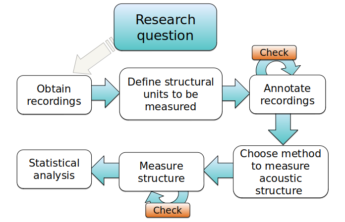
We can group warbleR functions according to the bioacoustic analysis stages.

 

2.1 Get and prepare recordings

The query_xc() function allows you to search and download sounds from the free access database Xeno-Canto. You can also convert .mp3 files to .wav, change the sampling rate of the files and correct corrupt files, among other functions.

Function	Description	Works.on	Output
check_wavs	verify if sound files can be read	multiple wave files	data frame
consolidate	consolidate sound files in a single folder	multiple wave files	data frame and wave files
fix_wavs	fix waves that cannot be read in R	multiple wave files	wave files
mp32wav	convert multiple mp3 files to wav format	multiple mp3 files	wave files
query_xc	Search and download mp3 files from Xeno-Canto	Scientific names/data frame	mp3 files
resample_est	resample wave objects in ext. selection tables	extended selection tables	extended selection tables
remove_channels	remove channels in multiple wave files	multiple wave files	wave files
remove_silence	remove silences in multiple wave files	multiple wave files	wave files
duration_wavs	measures duration in multiple wave files	multiple wave files	data frame
info_wavs	extract recording parameters from multiple wave files	multiple wave files	data frame

 

2.2 Annotating sound

It is recommended to make annotations in other programs and then import them into R (for example in Raven and import them with the Rraven package). However, warbleR offers some functions to facilitate manual or automatic annotation of sound files, as well as the subsequent manipulation:

Function	Description	Works.on	Output
auto_detec	automatic annotation of wave files	multiple wave files	data frame, images
optimize_auto_detec	Try different detection settings to optimize auto_detec detections	auto_detec output	data frame
freq_range	detect frequency range in selection tables	multiple wave files	data frame
tailor_sels	interactive tailoring of selections	selection tables	selection tables

 

2.3 Organize annotations

The annotations (or selection tables) can be manipulated and refined with a variety of functions. Selection tables can also be converted into the compact format extended selection tables:

Function	Description	Works.on	Output
auto_detec	automatic annotation of wave files	multiple wave files	data frame, images
optimize_auto_detec	Try different detection settings to optimize auto_detec detections	auto_detec output	data frame
freq_range	detect frequency range in selection tables	multiple wave files	data frame
tailor_sels	interactive tailoring of selections	selection tables	selection tables

 

2.4 Measure acoustic signal structure

Most warbleR functions are dedicated to quantifying the structure of acoustic signals listed in selection tables using batch processing. For this, 4 main measurement methods are offered:

1. Spectrographic parameters
2. Cross correlation
3. Dynamic time warping (DTW)
4. Statistical descriptors of cepstral coefficients

Most functions gravitate around these methods, or variations of these methods:

Function	Description	Works.on	Output
freq_range	detect frequency range in selection tables	multiple wave files	data frame
song_analysis	measures acoustic parameters at higher structural levels of organization	selection tables, ext. selection tables	data frame, selection tables
compare_methods	compare the performance of methods to measure acoustic structure	selection tables, ext. selection tables	images
freq_DTW	measures dynamic time warping (DTW) on dominant/fundamental frequency contours	selection tables, ext. selection tables	(di)similarity matrix, images
freq_ts	mesaures dominant/fundamental frequency contours	selection tables, ext. selection tables	data frame with frequency contours
inflections	measures number of inflections in frequency contours	data frame with frequency contours	data frame
mfcc_stats	measures statistical descriptors of Mel cepstral coefficients	selection tables, ext. selection tables	data frame
multi_DTW	measures dynamic time warping (DTW) on multiple contours	selection tables, ext. selection tables	(di)similarity matrix
sig2noise	measures signal-to-noise ratio	selection tables, ext. selection tables	selection tables, ext. selection tables
spectro_analysis	measures spectrographic parameters	selection tables, ext. selection tables	data frame
cross_correlation	measurec spectrographic cross-correlation	selection tables, ext. selection tables	(di)similarity matrix

 

Exercise

 

• Compare the performance of spectro_analysis() on the example ‘lbh_selec_table’ with “the argument ‘fast = TRUE’ vs ‘fast = FALSE’. What does this argument do and which seewave function might be involved?

 

2.5 Verify annotations

Functions are provided to detect inconsistencies in the selection tables or modify selection tables. The package also offers several functions to generate spectrograms showing the annotations, which can be organized by annotation categories. This allows you to verify if the annotations match the previously defined categories, which is particularly useful if the annotations were automatically generated.

Function	Description	Works.on	Output
check_sels	double-check selection tables	selection tables	selection tables
overlapping_sels	finds (time) overlapping selections	selection tables, ext. selection tables	selection tables, ext. selection tables
catalog	creates spectrogram catalog	selection tables, ext. selection tables	images
catalog2pdf	convert catalogs to .pdf	images	images
spectrograms	create spectrogram images	selection tables, ext. selection tables	images
full_spectrograms	create spectrograms of whole sound files	multiple wave files, selection tables, ext. selection tables	images
full_spectrogram2pdf	convert full spectrograms to .pfg	images	images

 

2.6 Visually inspection of annotations and measurements

Function	Description	Works.on	Output
snr_spectrograms	plots spectrograms highlighting areas where signal-to-noise ratio is measured	selection tables, ext. selection tables	images
spectrograms	create spectrogram images	selection tables, ext. selection tables	images
track_freqs	create spectrogram images including frequency contours	selection tables, ext. selection tables	images
plot_coordination	create schematic plots of coordinated signals	data frame	images
full_spectrograms	create spectrograms of whole sound files	multiple wave files, selection tables, ext. selection tables	images

 

2.7 Additional functions

Finally, warbleR offers functions to simplify the use of extended selection tables, organize large numbers of images with spectrograms and generate elaborated signal visualizations:

Function	Description	Works.on	Output
is_extended_selection_table	check if object is extended selection tables	data frame	TRUE/FALSE
is_selection_table	check if object is selection tables	data frame	TRUE/FALSE
catalog2pdf	convert catalogs to .pdf	images	images
move_imgs	moves images among folders	images	images
harmonic_track	measures harmonics with highest energy	wave object	data frame with frequency contours
map_xc	created maps from Xeno-Canto recordings	data frame	images
test_coordination	test statistical significance of vocal coordination	data frame	data frame
full_spectrogram2pdf	convert full spectrograms to .pfg	images	images
color_spectro	highlight signals with colors in a spectrogram	wave object	plot in R
freq_range_detec	detect frequency range in wave objetcs	wave object	data frame, plot in R
open_wd	open working directory
phylo_spectro	plots phylogenetic trees with spectrograms	selection tables	plot in R
read_wave	read wave files and wave objects	selection tables, ext. selection tables	wave object
sim_songs	simulate songs		wave object, wave file and selection table
tweak_spectro	creates mosaic plots with spectrograms with different display parameters	selection tables, ext. selection tables	images
warbleR_options	define global parameters for warbleR functions

 

Exercise

 

• Run the examples of the functions phylo_spectro() and color_spectro()

• Use the query_xc() and map_xc() functions to explore the geographical distribution of the Xeno-Canto recordings of a species (of bird) of your interest (if any!)

 

---

3 References

1. Araya-Salas M, G Smith-Vidaurre & M Webster. (2017). Assessing the effect of sound file compression and background noise on measures of acoustic signal structure. Bioacoustics 4622, 1–17
2. Araya-Salas M, Smith-Vidaurre G (2017) warbleR: An R package to streamline analysis of animal acoustic signals. Methods Ecol Evol 8:184–191.

 

---

Session information

R version 4.2.2 Patched (2022-11-10 r83330)
Platform: x86_64-pc-linux-gnu (64-bit)
Running under: Ubuntu 20.04.5 LTS

Matrix products: default
BLAS:   /usr/lib/x86_64-linux-gnu/blas/libblas.so.3.9.0
LAPACK: /usr/lib/x86_64-linux-gnu/lapack/liblapack.so.3.9.0

locale:
 [1] LC_CTYPE=es_ES.UTF-8       LC_NUMERIC=C              
 [3] LC_TIME=es_CR.UTF-8        LC_COLLATE=es_ES.UTF-8    
 [5] LC_MONETARY=es_CR.UTF-8    LC_MESSAGES=es_ES.UTF-8   
 [7] LC_PAPER=es_CR.UTF-8       LC_NAME=C                 
 [9] LC_ADDRESS=C               LC_TELEPHONE=C            
[11] LC_MEASUREMENT=es_CR.UTF-8 LC_IDENTIFICATION=C       

attached base packages:
[1] stats     graphics  grDevices utils     datasets  methods   base     

other attached packages:
[1] ggplot2_3.4.2        microbenchmark_1.4.9 warbleR_1.1.28      
[4] NatureSounds_1.0.4   knitr_1.42           seewave_2.2.0       
[7] tuneR_1.4.4         

loaded via a namespace (and not attached):
 [1] Rcpp_1.0.10       svglite_2.1.0     fftw_1.0-7        digest_0.6.31    
 [5] foreach_1.5.2     utf8_1.2.3        R6_2.5.1          signal_0.7-7     
 [9] evaluate_0.21     httr_1.4.6        pillar_1.9.0      rlang_1.1.1      
[13] rstudioapi_0.14   rmarkdown_2.21    webshot_0.5.4     stringr_1.5.0    
[17] htmlwidgets_1.5.4 RCurl_1.98-1.12   munsell_0.5.0     proxy_0.4-27     
[21] compiler_4.2.2    xfun_0.39         pkgconfig_2.0.3   systemfonts_1.0.4
[25] htmltools_0.5.5   tidyselect_1.2.0  tibble_3.2.1      dtw_1.23-1       
[29] codetools_0.2-19  fansi_1.0.4       viridisLite_0.4.2 dplyr_1.1.0      
[33] withr_2.5.0       shinyBS_0.61.1    MASS_7.3-58.2     bitops_1.0-7     
[37] brio_1.1.3        grid_4.2.2        jsonlite_1.8.4    gtable_0.3.3     
[41] lifecycle_1.0.3   magrittr_2.0.3    scales_1.2.1      cli_3.6.1        
[45] stringi_1.7.12    pbapply_1.7-0     farver_2.1.1      testthat_3.1.8   
[49] xml2_1.3.4        vctrs_0.6.2       generics_0.1.3    kableExtra_1.3.4 
[53] rjson_0.2.21      iterators_1.0.14  tools_4.2.2       glue_1.6.2       
[57] parallel_4.2.2    fastmap_1.1.1     yaml_2.3.7        colorspace_2.1-0 
[61] soundgen_2.5.3    rvest_1.0.3