R basics

 

Objetives

• Revisit the basic syntax and data structures in R

• Get familiar with documentation and help resources

 

1 What is R?

• A free Domain-Specific-Language (DSL) for statistics and data analysis
• A collection of over 19514 (may-12-2023) libraries
• A large and active community across industry and academia
• A way to talk “directly” to your computer

Historically:

• Based on the S Programming Language
• Around 20 years old (Lineage dates from 1975 - almost 40 years ago)

 

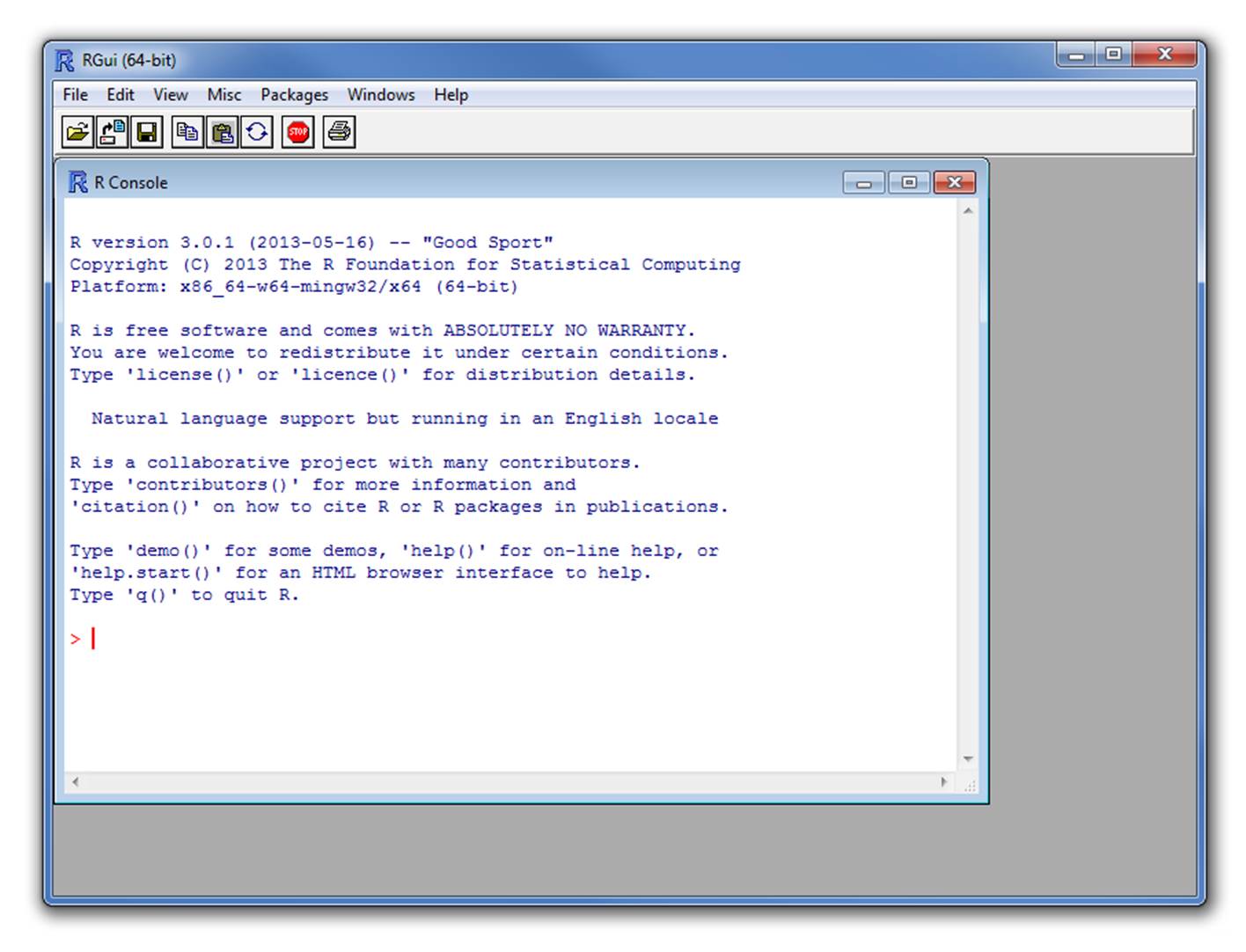
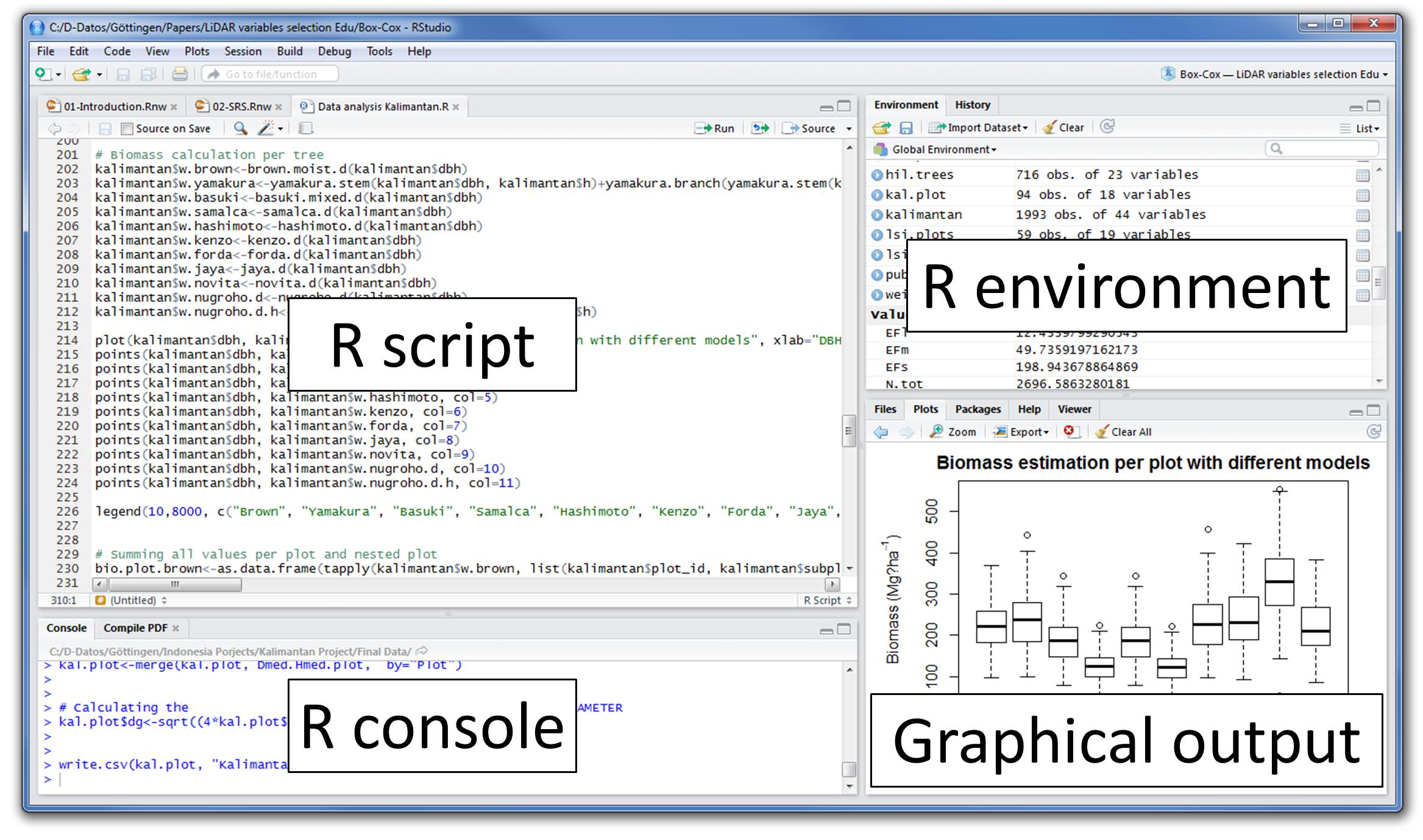
2 Rstudio

Integrated development environment (IDE) for R. Includes:

• A console
• Syntax-highlighting editor that supports direct code execution
• Tools for plotting, history, debugging and workspace management

---

3 Elements of the R language

• Vectors
• Lists
• Matrices
• Data Frames
• Functions (including operators)
• Attributes
• Tables
• Arrays
• Environments

Data structure

The basic data structure in R is the vector. There are two basic types of vectors: atomic vectors and lists.

They have three common properties:

• Type, typeof() (~ class/mode)
• Length, length() (number of elements)
• Attributes, attributes() (metadata)

They differ in the types of their elements: all elements of an atomic vector must be the same type, whereas the elements of a list can have different types.

	Homogeneous	Heterogeneous
1d	Atomic vector	List
2d	Matrix	Data frame
nd	Array

 

R has no 0-dimensional elements (scalars). Individual numbers or strings are actually vectors of length one.

Atomic vectors

Types of atomic vectors:

• Logical (boolean)
• Integer
• Numeric (double)
• Character

Vectors are built using c():

Code

x <- 1
x1 <- c(1)

all.equal(x, x1)
## [1] TRUE

class(x)
## [1] "numeric"

y <- "something"

class(y)
## [1] "character"

w <- 1L

class(w)
## [1] "integer"
 
z <- TRUE

class(z)
## [1] "logical"

q <- factor(1)

class(q)
## [1] "factor"

 

Vectors can only contain entries of the same type. Different types will be coerced to the most flexible type:

Code

v <- c(10, 11, 12, 13)

class(v)
## [1] "numeric"

is.integer(v)
## [1] FALSE

y <- c("Amazona", "Ara", "Eupsittula", "Myiopsitta")

class(y)
## [1] "character"

is.integer(y)
## [1] FALSE

x <- c(1,2,3, "Myiopsitta")

x
## [1] "1"          "2"          "3"          "Myiopsitta"

class(x)
## [1] "character"

 

Missing values are specified with NA, which is a logical vector of length 1. NA will always be coerced to the correct type if used inside c():

Code

v <- c(10, 11, 12, 13, NA)

class(v)
## [1] "numeric"

v <- c(letters[1:3], NA)

class(v)
## [1] "character"

 

Lists

Can contain objects of different classes and sizes. Lists are built using list():

Code

l <- list(ID = c("a", "b", "c", "d", "e"), 
          size = c(1, 2, 3, 4, 5), 
          observed = c(FALSE, TRUE, FALSE, FALSE, FALSE))

l

$ID
[1] "a" "b" "c" "d" "e"

$size
[1] 1 2 3 4 5

$observed
[1] FALSE  TRUE FALSE FALSE FALSE

Code

class(l)

[1] "list"

Code

str(l)

List of 3
 $ ID      : chr [1:5] "a" "b" "c" "d" ...
 $ size    : num [1:5] 1 2 3 4 5
 $ observed: logi [1:5] FALSE TRUE FALSE FALSE FALSE

… and dimensions:

Code

l <- list(ID = c("a", "b", "c", "d", "e"), 
          size = c(1, 2, 3, 4, 5, 6), 
          observed = c(FALSE, TRUE, FALSE, FALSE, FALSE), 
          l)

str(l)

List of 4
 $ ID      : chr [1:5] "a" "b" "c" "d" ...
 $ size    : num [1:6] 1 2 3 4 5 6
 $ observed: logi [1:5] FALSE TRUE FALSE FALSE FALSE
 $         :List of 3
  ..$ ID      : chr [1:5] "a" "b" "c" "d" ...
  ..$ size    : num [1:5] 1 2 3 4 5
  ..$ observed: logi [1:5] FALSE TRUE FALSE FALSE FALSE

Code

l2 <- list(l, l)

str(l2)

List of 2
 $ :List of 4
  ..$ ID      : chr [1:5] "a" "b" "c" "d" ...
  ..$ size    : num [1:6] 1 2 3 4 5 6
  ..$ observed: logi [1:5] FALSE TRUE FALSE FALSE FALSE
  ..$         :List of 3
  .. ..$ ID      : chr [1:5] "a" "b" "c" "d" ...
  .. ..$ size    : num [1:5] 1 2 3 4 5
  .. ..$ observed: logi [1:5] FALSE TRUE FALSE FALSE FALSE
 $ :List of 4
  ..$ ID      : chr [1:5] "a" "b" "c" "d" ...
  ..$ size    : num [1:6] 1 2 3 4 5 6
  ..$ observed: logi [1:5] FALSE TRUE FALSE FALSE FALSE
  ..$         :List of 3
  .. ..$ ID      : chr [1:5] "a" "b" "c" "d" ...
  .. ..$ size    : num [1:5] 1 2 3 4 5
  .. ..$ observed: logi [1:5] FALSE TRUE FALSE FALSE FALSE

 

Attributes

Objects can have attributes. Attributes allow to store metadata about the object. Attributes are kind of named lists. Attributes can be accessed individually with attr() or all at once (as a list) with attributes():

Code

y <- 1:10

mean(y)

[1] 5.5

Code

attr(y, "my_attribute") <- "This is an attribute"


attr(y, "my_attribute")

[1] "This is an attribute"

Code

str(y)

 int [1:10] 1 2 3 4 5 6 7 8 9 10
 - attr(*, "my_attribute")= chr "This is an attribute"

 

Most attributes are lost when modifying a vector:

Code

attributes(y[1])

NULL

 

The only attributes not lost are the three most important:

• Names, a character vector giving each element a name, described in names
• Dimensions
• Class

---

Code

w <- structure(c(a =1, b = 2), my_attribute = "This is not an apple")

attributes(w)

$names
[1] "a" "b"

$my_attribute
[1] "This is not an apple"

Code

attributes(w[1])

$names
[1] "a"

Code

class(w[1])

[1] "numeric"

 

Factors

Attributes are used to define factors. A factor is a vector that can contain only predefined values, and is used to store categorical data.

Factors are built on top of integer vectors using two attributes:

• class “factor”: makes them behave differently from regular integer vectors
• levels: defines the set of allowed values

Code

x <- factor(c("a", "b", "b", "a"))
x

[1] a b b a
Levels: a b

Code

levels(x)

[1] "a" "b"

Code

str(x)

 Factor w/ 2 levels "a","b": 1 2 2 1

 

Factors look like character vectors but they are actually integers:

Code

x <- factor(c("a", "b", "b", "a"))

c(x)

[1] a b b a
Levels: a b

 

Matrices

All entries are of the same type:

Code

m <- matrix(c(1, 2, 3, 11, 12, 13), nrow = 2)

dim(m)

[1] 2 3

Code

m

     [,1] [,2] [,3]
[1,]    1    3   12
[2,]    2   11   13

Code

class(m)

[1] "matrix" "array" 

Code

m <- matrix(c(1, 2, 3, 11, 12,"13"), nrow = 2)
m

     [,1] [,2] [,3]
[1,] "1"  "3"  "12"
[2,] "2"  "11" "13"

 

Data frames

Special case of lists. Can contain entries of different types:

Code

m <- data.frame(ID = c("a", "b", "c", "d", "e"), 
                size = c(1, 2, 3, 4, 5), 
                observed = c(FALSE, TRUE, FALSE, FALSE, FALSE))

dim(m)

[1] 5 3

Code

m

ID	size	observed
a	1	FALSE
b	2	TRUE
c	3	FALSE
d	4	FALSE
e	5	FALSE

Code

class(m)

[1] "data.frame"

Code

is.data.frame(m)

[1] TRUE

Code

is.list(m)

[1] TRUE

Code

str(m)

'data.frame':   5 obs. of  3 variables:
 $ ID      : chr  "a" "b" "c" "d" ...
 $ size    : num  1 2 3 4 5
 $ observed: logi  FALSE TRUE FALSE FALSE FALSE

 

But vectors should have the same length:

Code

m <- data.frame(ID = c("a", "b", "c", "d", "e"), 
                size = c(1, 2, 3, 4, 5, 6), 
                observed = c(FALSE, TRUE, FALSE, FALSE, FALSE))

Error in data.frame(ID = c("a", "b", "c", "d", "e"), size = c(1, 2, 3, : arguments imply differing number of rows: 5, 6

 

---

4 Data subsetting

Indexing

Elements within objects can be called by indexing. To subset a vector simply call the object position using square brackets:

Code

x <- c(1, 3, 4, 10, 15, 20, 50, 1, 6)

x[1]

[1] 1

Code

x[2]

[1] 3

Code

x[2:3]

[1] 3 4

Code

x[c(1,3)]

[1] 1 4

 

Elements can be removed in the same way:

Code

x[-1]

[1]  3  4 10 15 20 50  1  6

Code

x[-c(1,3)]

[1]  3 10 15 20 50  1  6

 

Matrices and data frames required 2 indices [row, column]:

Code

m <- matrix(c(1, 2, 3, 11, 12, 13), nrow = 2)

m[1, ]

[1]  1  3 12

Code

m[, 1]

[1] 1 2

Code

m[1, 1]

[1] 1

Code

m[-1, ]

[1]  2 11 13

Code

m[, -1]

     [,1] [,2]
[1,]    3   12
[2,]   11   13

Code

m[-1, -1]

[1] 11 13

Code

df <- data.frame(family = c("Psittacidae", "Trochilidae", 
                            "Psittacidae"), 
  genus = c("Amazona", "Phaethornis", "Ara"), 
    species = c("aestiva", "philippii", "ararauna"))

df

family	genus	species
Psittacidae	Amazona	aestiva
Trochilidae	Phaethornis	philippii
Psittacidae	Ara	ararauna

Code

df[1, ]

family	genus	species
Psittacidae	Amazona	aestiva

Code

df[, 1]

[1] "Psittacidae" "Trochilidae" "Psittacidae"

Code

df[1, 1]

[1] "Psittacidae"

Code

df[-1, ]

	family	genus	species
2	Trochilidae	Phaethornis	philippii
3	Psittacidae	Ara	ararauna

Code

df[, -1]

genus	species
Amazona	aestiva
Phaethornis	philippii
Ara	ararauna

Code

df[-1, -1]

	genus	species
2	Phaethornis	philippii
3	Ara	ararauna

Code

df[,"family"]

[1] "Psittacidae" "Trochilidae" "Psittacidae"

Code

df[,c("family", "genus")]

family	genus
Psittacidae	Amazona
Trochilidae	Phaethornis
Psittacidae	Ara

 

Lists require 1 index within double square brackets [[index]]:

Code

l <- list(ID = c("a", "b", "c", "d", "e"), size = c(1, 2, 3, 4, 5), observed = c(FALSE, TRUE, FALSE, FALSE, FALSE))

l[[1]]

[1] "a" "b" "c" "d" "e"

Code

l[[3]]

[1] FALSE  TRUE FALSE FALSE FALSE

 

Elements within lists can also be subset in the same string of code:

Code

l[[1]][1:2]

[1] "a" "b"

Code

l[[3]][2]

[1] TRUE

 

Exploring objects

Code

str(df)

'data.frame':   3 obs. of  3 variables:
 $ family : chr  "Psittacidae" "Trochilidae" "Psittacidae"
 $ genus  : chr  "Amazona" "Phaethornis" "Ara"
 $ species: chr  "aestiva" "philippii" "ararauna"

Code

names(df)

[1] "family"  "genus"   "species"

Code

dim(df)

[1] 3 3

Code

nrow(df)

[1] 3

Code

ncol(df)

[1] 3

Code

head(df)

family	genus	species
Psittacidae	Amazona	aestiva
Trochilidae	Phaethornis	philippii
Psittacidae	Ara	ararauna

Code

tail(df)

family	genus	species
Psittacidae	Amazona	aestiva
Trochilidae	Phaethornis	philippii
Psittacidae	Ara	ararauna

Code

table(df$genus)

    Amazona         Ara Phaethornis 
          1           1           1 

Code

typeof(df)

[1] "list"

Code

View(df)

 

Exercise

 

• Using the example data iris to create a data subset with only the observations of the species ‘setosa’

• Now create a data subset containing the observations of both ‘setosa’ and ‘versicolor’

• Also with iris create a data subset with the observations for which iris$Sepal.length is higher than 6

• How many observations have a sepal length higher than 6?

 

---

 

5 Functions

All functions are created by the function function() and follow the same structure:

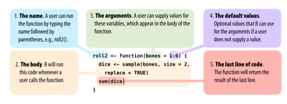
* Modified from Grolemund 2014  

R comes with many functions that you can use to do sophisticated tasks:

Code

# built in functions
bi <- builtins()

length(bi)

[1] 1375

Code

sample(bi, 10)

 [1] "bitwNot"              ".GlobalEnv"           "row.names.data.frame"
 [4] "%%"                   ".colSums"             "standardGeneric"     
 [7] "xtfrm.Date"           "<="                   "!.octmode"           
[10] "T"                   

 

Operators are functions:

Code

1 + 1

[1] 2

Code

'+'(1, 1)

[1] 2

Code

2 * 3

[1] 6

Code

'*'(2, 3)

[1] 6

 

Most commonly used R operators

Arithmetic operators:

                                 Operator       Description        
c.......addition..               "+"            "addition"         
c.......subtraction..            "-"            "subtraction"      
c.......multiplication..         "*"            "multiplication"   
c.......division..               "/"            "division"         
c....or.......exponent..         "^ or **"      "exponent"         
c..x....y....modulus..x.mod.y... "x %% y"       "modulus (x mod y)"
c..x.....y....integer.division.. "x %/% y"      "integer division" 

Code

1 - 2

[1] -1

Code

1 + 2

[1] 3

Code

2 ^ 2

[1] 4

 

Logical operators:

                                    Operator    Description               
c.......less.than..                 "<"         "less than"               
c........less.than.or.equal.to..    "<="        "less than or equal to"   
c.......greater.than..              ">"         "greater than"            
c........greater.than.or.equal.to.. ">="        "greater than or equal to"
c........exactly.equal.to..         "=="        "exactly equal to"        
c........not.equal.to..             "!="        "not equal to"            
c...x....Not.x..                    "!x"        "Not x"                   
c..x...y.....tx.OR.y..              "x | y"     "\tx OR y"                
c..x...y....x.AND.y..               "x & y"     "x AND y"                 
c..x..in..y....match..              "x %in% y"  "match"                   

Code

1 < 2 

[1] TRUE

Code

1 > 2 

[1] FALSE

Code

1 <= 2 

[1] TRUE

Code

1 == 2

[1] FALSE

Code

1 != 2

[1] TRUE

Code

1 > 2 

[1] FALSE

Code

5 %in% 1:6

[1] TRUE

Code

5 %in% 1:4

[1] FALSE

 

Most functions are vectorized:

Code

1:6 * 1:6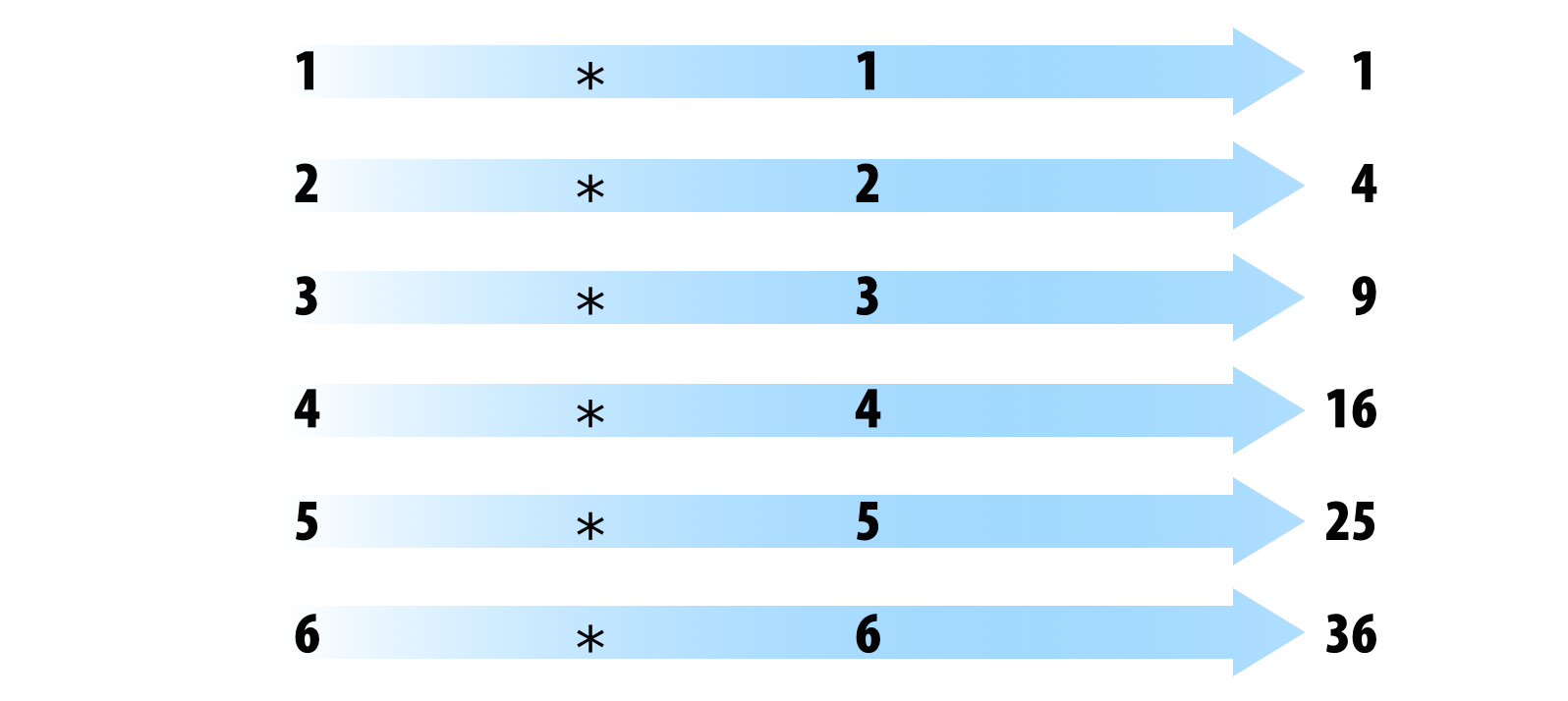

* Modified from Grolemund & Wickham 2017

 

[1]  1  4  9 16 25 36

Code

1:6 - 1:6

[1] 0 0 0 0 0 0

R recycles vectors of unequal length:

Code

1:6 * 1:5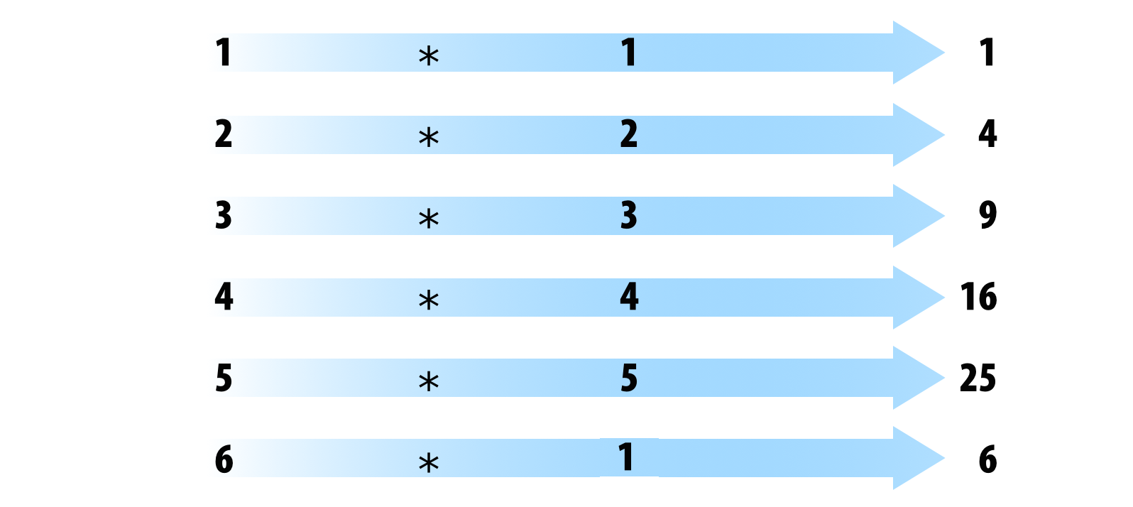

* Modified from Grolemund & Wickham 2017

 

Warning in 1:6 * 1:5: longitud de objeto mayor no es múltiplo de la longitud de
uno menor

[1]  1  4  9 16 25  6

Code

1:6 + 1:5

Warning in 1:6 + 1:5: longitud de objeto mayor no es múltiplo de la longitud de
uno menor

[1]  2  4  6  8 10  7

 

---

6 Style matters

Based on google’s R Style Guide

File names

File names should end in .R and, of course, be meaningful:

• GOOD: predict_ad_revenue.R
• BAD: foo.R

Object names

Variables and functions:

• Lowercase
• Use an underscore (_) (HW style)
• Generally, nouns for variables and verbs for functions
• Strive for names that are concise and meaningful (not always easy)
• Avoid using names of existing functions of variables

Code

  - GOOD: day_one: day_1, mean.day(),
  
  - BAD: dayOne, day1, firstDay_of.month, mean <- function(x) sum(x), c <- 10

 

Syntax

Spacing:

• Use spaces around operators and for argument within a function
• Always put a space after a comma, and never before (just like in regular English)
• Place a space before left parenthesis, except in a function call

Code

  - GOOD: 
          a <- rnorm(n = 10, sd = 10, mean = 1)
          tab.prior <- table(df[df$days.from.opt < 0, "campaign.id"])
          total <- sum(x[, 1])
          total <- sum(x[1, ])
          if (debug)
          mean(1:10)
          
  - BAD: 
         a<-rnorm(n=10,sd=10,mean=1)
         tab.prior <- table(df[df$days.from.opt<0, "campaign.id"])  # Needs spaces around '<'
         tab.prior <- table(df[df$days.from.opt < 0,"campaign.id"])  # Needs a space after the comma
         tab.prior<- table(df[df$days.from.opt < 0, "campaign.id"])  # Needs a space before <-
         tab.prior<-table(df[df$days.from.opt < 0, "campaign.id"])  # Needs spaces around <-
         total <- sum(x[,1])  # Needs a space after the comma
         total <- sum(x[ ,1])  # Needs a space after the comma, not before  
         if(debug) # Needs a space before parenthesis
         mean (1:10) # ) # Extra space before parenthesis

 

Curly braces:

• An opening curly brace should never go on its own line
• Closing curly brace should always go on its own line
• You may omit curly braces when a block consists of a single statement

Code

  - GOOD:
              if (is.null(ylim)) {
              ylim <- c(0, 0.06)
            }
                      
            if (is.null(ylim))
              ylim <- c(0, 0.06)
          
  - BAD:
            
         if (is.null(ylim)) ylim <- c(0, 0.06)
                    
         if (is.null(ylim)) {ylim <- c(0, 0.06)} 

         if (is.null(ylim)) {
           ylim <- c(0, 0.06)
           } 

 

Assigments:

• Use <-, not =

Code

  - GOOD:
         x <- 5 
          
  - BAD:
         x = 5

 

Commenting guidelines:

• Comment your code
• Entire commented lines should begin with # and one space
• Short comments can be placed after code preceded by two spaces, #, and then one space

Code

# Create histogram of frequency of campaigns by pct budget spent.
hist(df$pct.spent,
     breaks = "scott",  # method for choosing number of buckets
     main   = "Histogram: fraction budget spent by campaignid",
     xlab   = "Fraction of budget spent",
     ylab   = "Frequency (count of campaignids)")

 

General Layout and Ordering (google style):

• Copyright statement comment (?)
• Author comment
• File description comment, including purpose of program, inputs, and outputs
• source() and library() statements
• Function definitions
• Executed statements, if applicable (e.g., print, plot)

---

 

7 R documentation

Most R resources are extremely well documented. So the first source for help you should go to when writting R code is the R documention itself. All packages are documented in the same standard way. Getting familiar with the format can simplify things a lot.

Package documentation

 

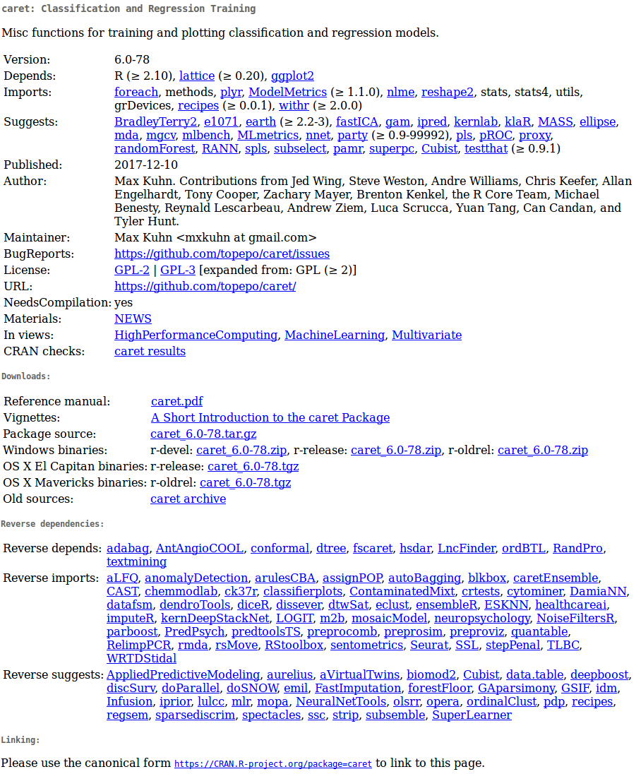
Reference manuals

Reference manuals are collections of the documentation for all functions in a package (only 1 per package):

• dynaSpec manual

• baRulho manual

 

Function documentation

All functions (default or from loaded packages) must have a documentation that follows a standard format:

Code

?mean

help("mean")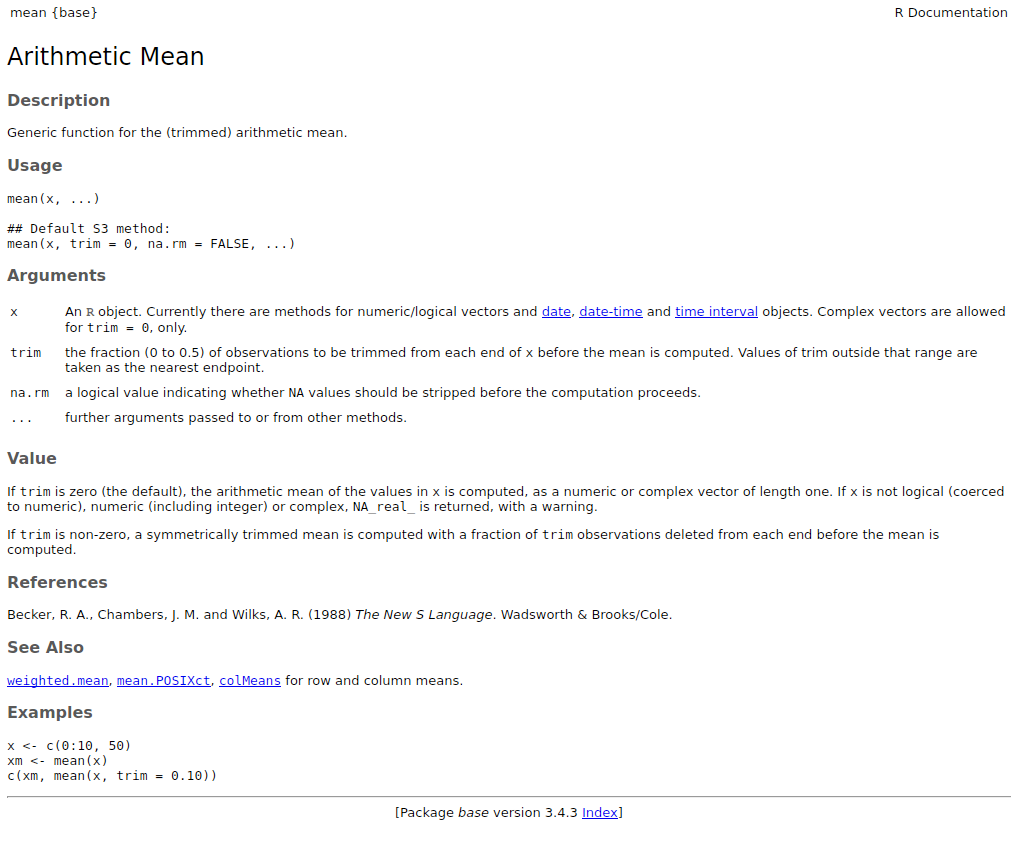

 

This documentation can also be shown in Rstudio by pressing F1 when the cursor is on the function name

 

If you don’t recall the function name try apropos():

Code

apropos("mean")

 [1] ".colMeans"     ".rowMeans"     "colMeans"      "kmeans"       
 [5] "mean"          "mean.Date"     "mean.default"  "mean.difftime"
 [9] "mean.POSIXct"  "mean.POSIXlt"  "rowMeans"      "weighted.mean"

 

Vignettes

Vignettes are illustrative documents or study cases detailing the use of a package (optional, can be several per package).

Vignettes can be called directly from R:

Code

vgn <- browseVignettes() 

Code

vignette()

They should also be listed in the package CRAN page.

 

Demonstrations

Packages may also include extended code demonstrations (‘demos’). To list demos in a package run demo("package name"):

Code

demo(package="stats")

# call demo directly
demo("nlm")

 

Exercise

 

• What does the function cut() do?

• What is the breaks argument in cut() used for?

• Run the first 4 lines of code in the examples supplied in the cut() documentation

• How many vignettes does the package warbleR has?

 

---

8 References

• Advanced R, H Wickham
• Google’s R Style Guide
  
• Hands-On Programming with R (Grolemund, 2014)